methylTFR: Quantification of DNA Methylation Signatures in Transcription Factor Binding Sites

Introduction

DNA methylation can modulate transcription factor (TF) binding, particularly when occurring within transcription factor binding sites (TFBS). methylTFR is an R package that identifies DNA methylation signatures at TFBS using whole-genome bisulfite sequencing (WGBS) data.

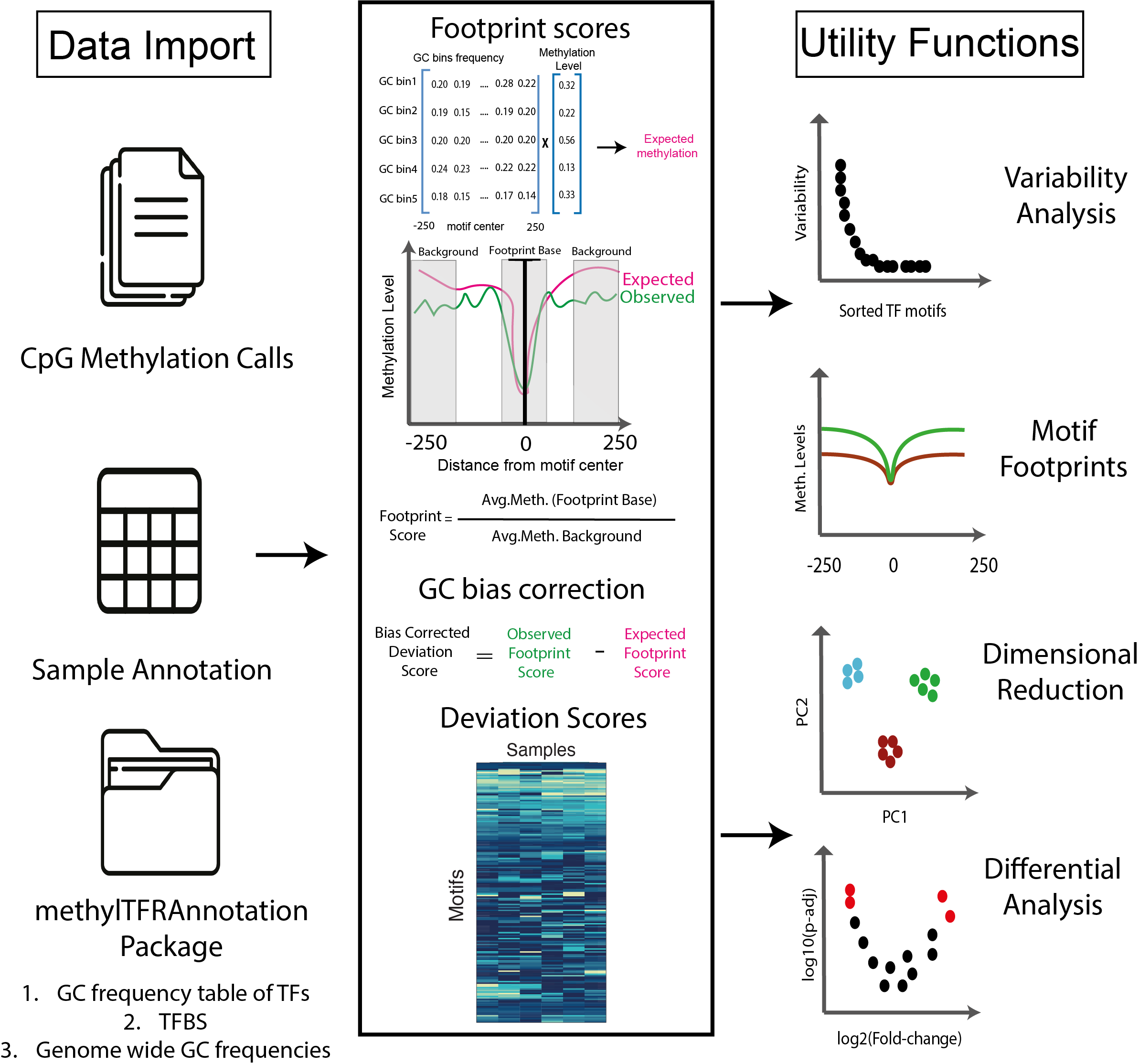
For each sample, methylation levels are first aggregated across all genomic regions corresponding to TFBS. This yields the observed deviation, which captures the raw signal of methylation enrichment or depletion for each TF. To account for sequence composition biases, methylTFR then estimates an expected deviation using genomic background models derived from TF motif GC content and genome-wide GC frequency. This deviation matrix provides a compact and interpretable representation of TFBS methylation across samples, suitable for downstream analyses such as dimensionality reduction (e.g., PCA, UMAP), clustering, differential testing, and visualization of TF-specific methylation footprints.

Installation

You can install the stable release of methylTFR from Bioconductor using:

if (!requireNamespace("BiocManager", quietly = TRUE)) {
  install.packages("BiocManager")
}

BiocManager::install("methylTFR")

To install the development version directly from GitHub:

if (!requireNamespace("remotes", quietly = TRUE)) {
  install.packages("remotes")
}
remotes::install_github("EpigenomeInformatics/methylTFR")

Getting Started

To get started with methylTFR, load the package and its dependencies:

library(methylTFR)
#> Loading required package: data.table
#> Warning: multiple methods tables found for 'sort'
#> Warning: multiple methods tables found for 'sort'
#> Warning: replacing previous import 'S4Arrays::read_block' by
#> 'DelayedArray::read_block' when loading 'HDF5Array'
#> Warning: replacing previous import 'S4Arrays::read_block' by
#> 'DelayedArray::read_block' when loading 'SummarizedExperiment'
#> Warning: multiple methods tables found for 'sort'
#> 
#> Attaching package: 'methylTFR'
#> The following objects are masked from 'package:base':
#> 
#>     cbind, rbind

Read a Sample File

The read_methylome() function is used to import single-sample DNA methylation data into a GRanges object.
It supports several common file formats, including EPP, ALLC, BisSNP, bismarkCytosine, bismarkcov, and ENCODE.

You can optionally filter out low-coverage sites using the cov_threshold parameter (default = 1), which excludes positions with insufficient read support.

Below is an example of reading an example EPP-formatted file provided in the package:

epp_path <- system.file("extdata", "epp.tsv.gz", package = "methylTFR")
epp <- read_methylome(epp_path, "EPP")
epp
#> GRanges object with 6 ranges and 2 metadata columns:
#>       seqnames          ranges strand |     score  coverage
#>          <Rle>       <IRanges>  <Rle> | <numeric> <numeric>
#>   [1]     chr1 3010957-3010958      + |     1.000        27
#>   [2]     chr1 3010959-3010960      - |     0.500         7
#>   [3]     chr1 3010971-3010972      + |     1.000        20
#>   [4]     chr1 3010973-3010974      - |     0.500        20
#>   [5]     chr1 3011025-3011026      + |     0.814        70
#>   [6]     chr1 3011027-3011028      - |     0.500       100
#>   -------
#>   seqinfo: 1 sequence from an unspecified genome; no seqlengths

Annotation Resources

We provide precomputed TFBS-based annotation data for the human genome (hg38), which is required by methylTFR to compute expected deviations.
This includes transcription factor binding sites, GC content windows, and motif GC frequency models.

You can download the hg38-compatible annotation package from the following AWS-hosted archive:

Download methylTFRAnnotationsHg38.tar.gz

Optionally, you can create a customized annotation package for use with methylTFR using the methylTFRAnnotationBuilder package available on GitHub.

Input Data

methylTFR relies on several precomputed annotation resources to estimate expected methylation levels at transcription factor binding sites (TFBS). These annotations include:

GC distribution (gcdist_subset): Genome-wide GC content distribution around cytosines, used to model methylation expectations.
Motif GC frequency (BATF_gcfreqs): GC frequency profile specific to the BATF motif across TFBS, used to correct for sequence composition bias.
TF binding sites (BATF_tf_bindsites): A GRanges object containing the genomic coordinates of BATF binding sites.
Example methylation data (example_data): A small subset of methylation calls in EPP format, read using the read_methylome() function, provided for demonstration purposes.

The following code loads these example datasets and displays the first few entries:

# Load the data
load(system.file("extdata", "gcdist_subset.rda", package = "methylTFR"))
load(system.file("extdata", "BATF_gcfreqs.rda", package = "methylTFR"))
load(system.file("extdata", "BATF_tf_bindsites.rda", package = "methylTFR"))
load(system.file("extdata", "example_data.rda", package = "methylTFR"))


# Check the data
head(gcdist)
#> GRanges object with 6 ranges and 2 metadata columns:
#>       seqnames      ranges strand |   GC_bias    GC_bin
#>          <Rle>   <IRanges>  <Rle> | <numeric> <integer>
#>   [1]     chr1 10471-10500      * |  0.866667         5
#>   [2]     chr1 10591-10620      * |  0.633333         5
#>   [3]     chr1 10621-10650      * |  0.800000         5
#>   [4]     chr1 13051-13080      * |  0.700000         5
#>   [5]     chr1 13261-13290      * |  0.666667         5
#>   [6]     chr1 13291-13320      * |  0.600000         5
#>   -------
#>   seqinfo: 22 sequences from an unspecified genome
head(gcfreqs$BATF[, 1:5])
#>           [,1]      [,2]      [,3]      [,4]      [,5]
#> [1,] 0.1398816 0.1394321 0.1386829 0.1366599 0.1361355
#> [2,] 0.1538173 0.1546415 0.1580880 0.1591369 0.1620589
#> [3,] 0.1962239 0.2001199 0.1965985 0.1973477 0.1916536
#> [4,] 0.2734697 0.2706226 0.2724957 0.2718214 0.2769911
#> [5,] 0.2366075 0.2351839 0.2341350 0.2350341 0.2331610
head(tf_bindsites)
#> $BATF
#> GRanges object with 268717 ranges and 1 metadata column:
#>            seqnames            ranges strand |     score
#>               <Rle>         <IRanges>  <Rle> | <numeric>
#>        [1]     chr1       47430-47840      + |   16.7687
#>        [2]     chr1       57232-57642      + |   13.2598
#>        [3]     chr1       93216-93626      + |   14.9499
#>        [4]     chr1       96525-96935      + |   13.6042
#>        [5]     chr1       99285-99695      + |   13.9006
#>        ...      ...               ...    ... .       ...
#>   [268713]     chrY 57027771-57028181      - |   15.5241
#>   [268714]     chrY 57050236-57050646      - |   14.0836
#>   [268715]     chrY 57074721-57075131      - |   13.8672
#>   [268716]     chrY 57080582-57080992      - |   13.3138
#>   [268717]     chrY 57166552-57166962      - |   13.3138
#>   -------
#>   seqinfo: 24 sequences from an unspecified genome; no seqlengths
head(msites)
#> GRanges object with 6 ranges and 2 metadata columns:
#>       seqnames      ranges strand |     score  coverage
#>          <Rle>   <IRanges>  <Rle> | <numeric> <integer>
#>   [1]     chr1 10471-10472      - |         1         9
#>   [2]     chr1 10608-10609      + |         0         2
#>   [3]     chr1 10609-10610      - |         1         1
#>   [4]     chr1 10616-10617      + |         0         2
#>   [5]     chr1 10617-10618      - |         1         1
#>   [6]     chr1 10619-10620      + |         0         2
#>   -------
#>   seqinfo: 170 sequences from an unspecified genome; no seqlengths

Compute Deviation Score for a Single Sample and Single Motif

The computeDeviation() function calculates the deviation score for a specific transcription factor (TF) motif in a single sample. It compares the observed methylation at TF binding sites (TFBS) to the expected methylation derived from GC frequency models.

This example uses the BATF motif and the example methylation dataset loaded earlier. The methylation data must first be binned by GC content using addGCBintoMethylome() before computing the deviation.

# Add GC bins to methylation data
bin_meth <- addGCBintoMethylome(msites, gcdist, ignoreStrand = TRUE)
bin_meth
#>      gcbin avg_mscore
#> [1,]     1  0.5315789
#> [2,]     2  0.6466688
#> [3,]     3  0.7217031
#> [4,]     4  0.7091566
#> [5,]     5  0.7838198

# Compute deviation score for BATF motif
deviation_score <- computeDeviation(
    motif = "BATF",
    msites = msites,
    tf_bindsites = tf_bindsites,
    gcfreqs = gcfreqs,
    enhancer = NULL,
    ignoreStrand = TRUE,
    binMsites = bin_meth
)

# View the result
deviation_score
#>         dev   exp_dev
#>       <num>     <num>
#> 1: 1.743674 0.9835985

Run methylTFR on multiple samples and motifs

The methylTFR package provides a run_methyltfr function to run the analysis on multiple samples and motif sites. You need to download the annotation package for the human genome (hg38) and place it in your working directory.

library(methylTFRAnnotationHg38) # annotation package for hg38

gcfreqs <- getGCfreq(motifSet = "jaspar2020")
gc_dist <- getGenomeGC("hg38")
tf_bindsites <- getTFbindsites(motifSet = "jaspar2020")

sample_dir <- file.path("samples_dir")
sample_ann <- "samples.tsv" # should contain column name bedFile

# deviation score matrix
deviations <- run_methyltfr(sample_ann, # sample annotation file
    sample_dir, # where the EPP files are
    threads = 8, # number of threads
    chunkSize = 10, # number of chunks to process
    sampleColName = "bedFile", # column name for EPP file paths in sample_ann
    tf_bindsites = tf_bindsites, # TF binding sites
    gcfreqs = gcfreqs, # GC frequency
    gc_dist = gc_dist, # GC distribution
    filetype = "EPP" # file type
)

Motif Footprinting

The methylTFR package provides a plotMotifFootprint function to visualize the methylation footprint of a specific TF motif per sample.

library(ggplot2)
load(system.file("extdata", "msites_sub.rda", package = "methylTFR"))
load(system.file("extdata", "gcdist_BATF.rda", package = "methylTFR"))

p <- plotMotifFootprint(
    motif = "BATF",
    tf_bindsites = tf_bindsites,
    gc_dist = gcdist,
    gcfreqs = gcfreqs,
    msites = msites_sub,
    sample_name = "ExampleSample",
    enhancer = NULL,
    method = "division"
)
p
#> Warning: Removed 112 rows containing missing values or values outside the scale range
#> (`geom_line()`).

Expected vs Observed Footprint

To visually assess how observed methylation patterns compare with expected profiles at transcription factor binding sites (TFBS), methylTFR provides the plotExpectedFootprint() function. This generates a footprint plot for a given motif in a single sample, allowing you to inspect local methylation behavior relative to GC-derived expectations.

In the example below, we visualize the methylation footprint for the BATF motif using the included example data.

# Generate footprint plot for BATF
p <- plotExpectedFootprint(
    motif = "BATF",
    tf_bindsites = tf_bindsites,
    msites = msites_sub,
    sample_name = "ExampleSample",
    gc_dist = gcdist,
    gcfreqs = gcfreqs,
    enhancer = NULL,
    returnPlotData = FALSE
)

p

Differential TF Activity Analysis

To assess differential TF activity between two groups of samples, methylTFR provides the differential_deviation_test() function. This function computes the observed and expected deviation scores for each TF motif across the specified groups, enabling statistical testing to identify differentially active TFs.

This is how methylTFRdeviations object is looked like:

load(system.file("extdata", "tc_mem.rda", package = "methylTFR"))
load(system.file("extdata", "tc_naive.rda", package = "methylTFR"))
devs <- cbind(tc_mem, tc_naive)
devs
#> class: methylTFRdeviations 
#> dim: 10 10 
#> metadata(0):
#> assays(2): deviations z
#> rownames(10): FOXF2 FOXD1 ... RORA RORA(var.2)
#> rowData names(1): motifs
#> colnames(10): Tc-Mem_OP_S5_Long_D1.bedGraph.bed
#>   Tc-Mem_OP_S4_Long_D60.bedGraph.bed ...
#>   Tc-Naive_OP_S4_Long_D1.bedGraph.bed
#>   Tc-Naive_OP_S3_High_D1.bedGraph.bed
#> colData names(4): CommonMinID condition cell_type bedFile

# Construct group labels from sample names
get_groupname <- function(x) {
    return(unlist(strsplit(x, split = "_"))[1])
}
groups <- sub(
    ".bedGraph", "",
    unlist(lapply(
        FUN = get_groupname,
        X = colnames(devs)
    ))
)
table(groups)
#> groups
#>   Tc-Mem Tc-Naive 
#>        5        5

# Run the differential deviation test
tc_result <- differential_deviation_test(
    deviations = devs,
    groups = groups,
    alternative = "two.sided",
    parametric = TRUE,
    padjMethod = "BH"
)

# View the results
head(tc_result)
#>                  motifs      p_value p_value_adjusted mean_difference
#> FOXF2             FOXF2 1.694736e-02     0.0355317162      0.02920759
#> FOXD1             FOXD1 3.644010e-01     0.4555013119      0.01081636
#> IRF2               IRF2 1.873667e-03     0.0093683362      0.03414276
#> MZF1(var.2) MZF1(var.2) 1.776586e-02     0.0355317162      0.01850831
#> MAX::MYC       MAX::MYC 1.078111e-05     0.0001078111      0.09341429
#> PPARG             PPARG 3.996324e-03     0.0133210805      0.03428684

Session Information

sessionInfo()
#> R version 4.4.1 (2024-06-14)
#> Platform: x86_64-conda-linux-gnu
#> Running under: Debian GNU/Linux 11 (bullseye)
#> 
#> Matrix products: default
#> BLAS/LAPACK: /icbb/projects/share/software/packages/miniconda3/envs/igunduz/lib/libopenblasp-r0.3.21.so;  LAPACK version 3.9.0
#> 
#> locale:
#>  [1] LC_CTYPE=en_US.UTF-8       LC_NUMERIC=C              
#>  [3] LC_TIME=en_US.UTF-8        LC_COLLATE=en_US.UTF-8    
#>  [5] LC_MONETARY=en_US.UTF-8    LC_MESSAGES=en_US.UTF-8   
#>  [7] LC_PAPER=en_US.UTF-8       LC_NAME=C                 
#>  [9] LC_ADDRESS=C               LC_TELEPHONE=C            
#> [11] LC_MEASUREMENT=en_US.UTF-8 LC_IDENTIFICATION=C       
#> 
#> time zone: Europe/Berlin
#> tzcode source: system (glibc)
#> 
#> attached base packages:
#> [1] stats     graphics  grDevices utils     datasets  methods   base     
#> 
#> other attached packages:
#> [1] ggplot2_4.0.1     methylTFR_0.99.0  data.table_1.17.2 BiocStyle_2.34.0 
#> 
#> loaded via a namespace (and not attached):
#>  [1] SummarizedExperiment_1.32.0 gtable_0.3.6               
#>  [3] xfun_0.52                   bslib_0.9.0                
#>  [5] htmlwidgets_1.6.4           rhdf5_2.46.1               
#>  [7] Biobase_2.62.0              lattice_0.22-5             
#>  [9] generics_0.1.4              rhdf5filters_1.14.1        
#> [11] vctrs_0.6.5                 tools_4.4.1                
#> [13] bitops_1.0-9                parallel_4.4.1             
#> [15] stats4_4.4.1                tibble_3.2.1               
#> [17] pkgconfig_2.0.3             R.oo_1.27.1                
#> [19] Matrix_1.6-1.1              RColorBrewer_1.1-3         
#> [21] S7_0.2.0                    desc_1.4.3                 
#> [23] S4Vectors_0.40.1            lifecycle_1.0.4            
#> [25] GenomeInfoDbData_1.2.13     stringr_1.5.1              
#> [27] compiler_4.4.1              farver_2.1.2               
#> [29] textshaping_0.4.0           GenomeInfoDb_1.42.3        
#> [31] htmltools_0.5.8.1           sass_0.4.10                
#> [33] RCurl_1.98-1.13             yaml_2.3.10                
#> [35] pillar_1.10.2               pkgdown_2.2.0              
#> [37] crayon_1.5.3                jquerylib_0.1.4            
#> [39] R.utils_2.13.0              DelayedArray_0.28.0        
#> [41] cachem_1.1.0                abind_1.4-8                
#> [43] tidyselect_1.2.1            digest_0.6.37              
#> [45] stringi_1.8.4               dplyr_1.1.3                
#> [47] bookdown_0.43               labeling_0.4.3             
#> [49] fastmap_1.2.0               grid_4.4.1                 
#> [51] cli_3.6.3                   SparseArray_1.2.4          
#> [53] magrittr_2.0.3              logger_0.4.0               
#> [55] S4Arrays_1.6.0              dichromat_2.0-0.1          
#> [57] withr_3.0.2                 UCSC.utils_1.2.0           
#> [59] scales_1.4.0                rmarkdown_2.29             
#> [61] XVector_0.42.0              httr_1.4.7                 
#> [63] matrixStats_1.1.0           ragg_1.3.3                 
#> [65] R.methodsS3_1.8.2           HDF5Array_1.30.1           
#> [67] evaluate_1.0.3              knitr_1.50                 
#> [69] GenomicRanges_1.54.1        IRanges_2.36.0             
#> [71] rlang_1.1.4                 glue_1.7.0                 
#> [73] BiocManager_1.30.25         BiocGenerics_0.52.0        
#> [75] jsonlite_2.0.0              R6_2.6.1                   
#> [77] Rhdf5lib_1.28.0             MatrixGenerics_1.14.0      
#> [79] systemfonts_1.2.3           fs_1.6.6                   
#> [81] zlibbioc_1.52.0

Irem B. Gündüz, Sarath Kumar Murugan, Fabian Muller

2026-06-10