Analysis of single-cell
ATAC-seq
data using ChrAccR
data using ChrAccR
Fabian Mueller
2026-09-28
Source:vignettes/singlecell.Rmd
singlecell.Rmd
Introduction
Single-cell ATAC datasets can be analyzed much like bulk datasets
using ChrAccR. Please refer to the main vignette for a
guide on how to analyze bulk data. First, let us load the package and
prepare the plot style used in the remainder of this vignette.
Loading the example data
In addition to bulk data, the ChrAccRex data package
contains a small example single-cell ATAC-seq datasets. If you haven’t
already installed ChrAccRex use
devtools::install_github("EpigenomeInformatics/ChrAccRex")The example data used in this vignette was designed for illustrating
the functionality of ChrAccR rather than a full analysis.
It contains ATAC-seq data for a subset of 3000 cells derived from
peripheral blood and bone marrow samples describing human hematopoiesis
(Granja et al.
2019) and it focuses on only a subset of the human genome
(chromosomes 1 and 21). It can be loaded using:
dsa <- ChrAccRex::loadExample("dsAtacSc_hema_example")
DsATACsc data structure
Analysis of single-cell datasets in ChrAccR works much
like bulk datasets. ChrAccR implements a special subclass
of DsATAC for storing and operating on single-cell
datasets. This subclass is called DsATACsc. The main
difference is that the ‘’samples’’ are actually individual cells:
dsa> Single-cell DsATAC chromatin accessibility dataset
> [in memory object]
> contains:
> * 3000 samples: BMMC_D5T1_AAACTCGCAAATTGAG-1, BMMC_D5T1_AAACTGCCACCAAGGA-1, BMMC_D5T1_AAACTGCCAGTAAGAT-1, BMMC_D5T1_AAACTGCCAGTCCTGG-1, BMMC_D5T1_AAACTGCCATTACTTC-1, ...
> * fragment data for 3000 samples
> * 3 region types: tiling5kb, promoter, .peaks.itlsi
> * * 59477 regions of type tiling5kb
> * * 2318 regions of type promoter
> * * 56045 regions of type .peaks.itlsiQuality control statistics
The annotation table stored with the dataset object can contain a number of statistics that are useful for cell quality control and filtering.
cell_anno <- getSampleAnnot(dsa)
colnames(cell_anno)
> [1] ".sampleId" "cellId"
> [3] "cellBarcode" "sampleId"
> [5] "cellType" "platform"
> [7] "geoId" "fragmentFile"
> [9] "label_granja" "nFrags"
> [11] ".tssEnrichment_unsmoothed" ".tssEnrichment"
cutoff_tss <- 15
cutoff_nfrags <- 4000
ggplot(cell_anno) + aes(x=log10(nFrags), y=.tssEnrichment) +
    geom_hline(yintercept=cutoff_tss, color="green") +
    geom_vline(xintercept=log10(cutoff_nfrags), color="green") +
    geom_point(size=0.5) + facet_wrap(~sampleId)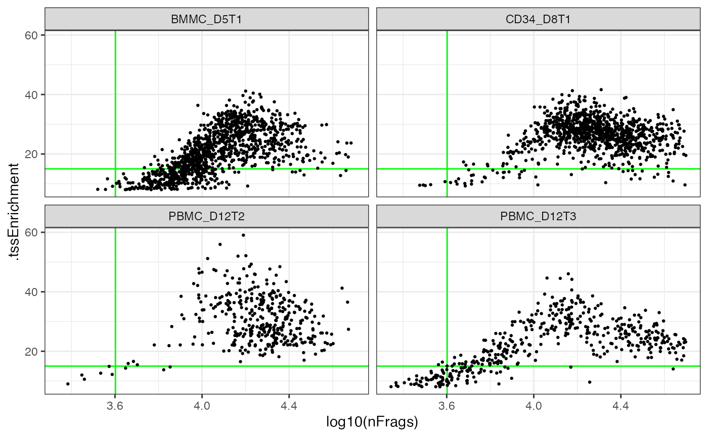
dsa_filtered <- dsa[cell_anno[,".tssEnrichment"] > cutoff_tss & cell_anno[,"nFrags"] > cutoff_nfrags]
length(getSamples(dsa))
> [1] 3000
length(getSamples(dsa_filtered))> [1] 2527Exploratory analysis
Dimension reduction and clustering using iterative LSI
In order to obtain a low dimensional representation of single-cell
ATAC datasets in terms of principal components and UMAP coordinates, we
recommend an iterative application of the Latent Semantic Indexing
approach (Cusanovich et al. 2018)
described in (Granja et al. 2019). This
approach also identifies cell clusters and a peak set that represents a
consensus peak set of cluster peaks in a given dataset. In brief, in an
initial iteration clusters are identified based on the most accessible
regions (e.g. genomic tiling regions). Here, the counts are first
normalized using the term frequency–inverse document frequency (TF-IDF)
transformation and singular values are computed based on these
normalized counts in selected regions (i.e. the most accessible regions
in the initial iteration). Clusters are identified based on the singular
values using Louvain clustering (as implemented in the
Seurat package). Peak calling is then performed on the
aggregated insertion sites from all cells of each cluster (using MACS2)
and a union/consensus set of peaks uniform-length non-overlapping peaks
is selected. In a second iteration, the peak regions whose
TF-IDF-normalized counts which exhibit the most variability across the
initial clusters provide the basis for a refined clustering using
derived singular values. In the final iteration, the most variable peaks
across the refined clusters are identified as the final peak set and
singular values are computed again. Based on these final singular values
UMAP coordinates are computed for low-dimensional projection.
# requires MACS2 for peak calling
itlsi <- iterativeLSI(dsa, it0regionType="tiling5kb", it0clusterResolution=0.4, it1clusterResolution=0.4, it2clusterResolution=0.4)
# load precomputed object
itlsi <- ChrAccRex::loadExample("itLsiObj_hema_example")
The output object includes the final singular values/principal
components (itlsi$pcaCoord), the low-dimensional
coordinates (itlsi$umapCoord), the final cluster assignment
of all cells (itlsi$clustAss), the complete, unfiltered
initial cluster peak set (itlsi$clusterPeaks_unfiltered) as
well as the final cluster-variable peak set
(itlsi$regionGr):
str(itlsi$pcaCoord)> num [1:3000, 1:50] 0.0249 0.0242 0.023 0.0228 0.0232 ...
> - attr(*, "dimnames")=List of 2
> ..$ : chr [1:3000] "BMMC_D5T1_AAACTCGCAAATTGAG-1" "BMMC_D5T1_AAACTGCCACCAAGGA-1" "BMMC_D5T1_AAACTGCCAGTAAGAT-1" "BMMC_D5T1_AAACTGCCAGTCCTGG-1" ...
> ..$ : chr [1:50] "PC1" "PC2" "PC3" "PC4" ...
> - attr(*, "percVar")= num [1:50] 32.62 4.68 2.57 2.14 2.04 ...
> - attr(*, "PCAclass")= chr "PCcoord"
> - attr(*, "PCAmethod")= chr "irldba_svd"
> - attr(*, "SVD_D")= num [1:50, 1:50] 1.17 0 0 0 0 ...
> - attr(*, "SVD_U")= num [1:50000, 1:50] 0.00141 0.0013 0.00827 0.00411 0.0078 ...
> - attr(*, "SVD_V")= num [1:3000, 1:50] 0.0212 0.0206 0.0196 0.0194 0.0198 ...
str(itlsi$umapCoord)> num [1:3000, 1:2] -7.35 -7 -7.56 -5.6 -7.5 ...
> - attr(*, "dimnames")=List of 2
> ..$ : chr [1:3000] "BMMC_D5T1_AAACTCGCAAATTGAG-1" "BMMC_D5T1_AAACTGCCACCAAGGA-1" "BMMC_D5T1_AAACTGCCAGTAAGAT-1" "BMMC_D5T1_AAACTGCCAGTCCTGG-1" ...
> ..$ : chr [1:2] "UMAP1" "UMAP2"
str(itlsi$clustAss)> Factor w/ 7 levels "c0","c1","c2",..: 1 1 1 5 1 4 4 4 1 1 ...
> - attr(*, "names")= chr [1:3000] "BMMC_D5T1_AAACTCGCAAATTGAG-1" "BMMC_D5T1_AAACTGCCACCAAGGA-1" "BMMC_D5T1_AAACTGCCAGTAAGAT-1" "BMMC_D5T1_AAACTGCCAGTCCTGG-1" ...
length(itlsi$clusterPeaks_unfiltered)> [1] 300997
length(itlsi$regionGr)> [1] 50000You can use the resulting low-dimensional projections to characterize variability in your dataset according to various cell annotions. Here, we visualize the final cluster assignment …
df <- data.frame(
  itlsi$umapCoord,
  cluster = itlsi$clustAss,
  cellId = rownames(itlsi$umapCoord),
  sampleSource = getSampleAnnot(dsa)[,"cellType"],
  stringsAsFactors = FALSE
)

ggplot(df, aes(x=UMAP1, y=UMAP2, color=cluster)) + geom_point(size=0.25)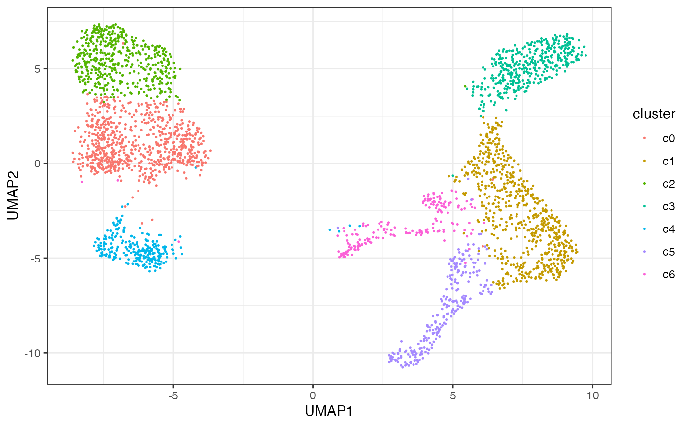
… as well as the annotated sample source:
ggplot(df, aes(x=UMAP1, y=UMAP2, color=sampleSource)) + geom_point(size=0.25)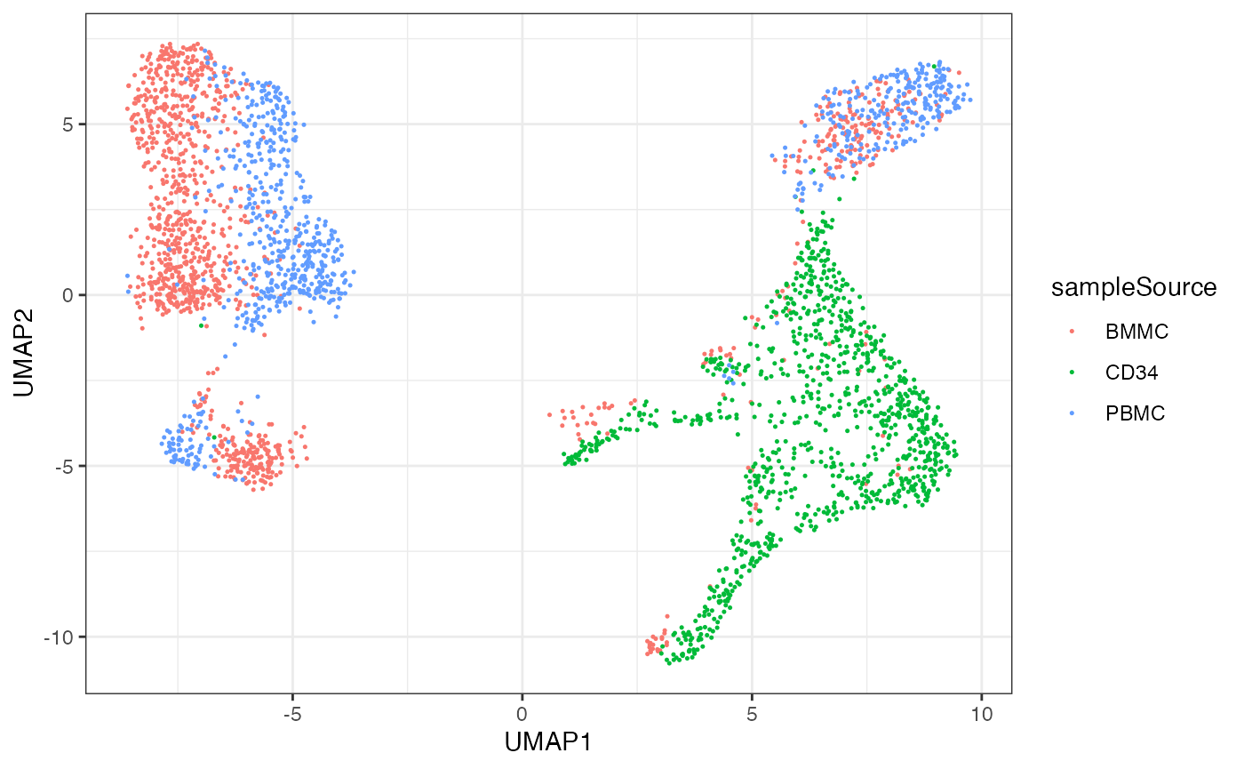
chromVAR deviations
We utilize chromVAR in order to determine the
genome-wide TF motif activity for each cell (Schep et al. 2017). You can use the
low-dimensional projection in order to visualize variability in TF motif
accessibility across all cells in the manifold.
cvRes <- getChromVarDev(dsa, ".peaks.itlsi", motifs="jaspar2018")
devZ <- t(chromVAR::deviations(cvRes))

motifNames <- c("MA0036.3_GATA2", "MA0652.1_IRF8", "MA0102.3_CEBPA", "MA0690.1_TBX21")
df_with_cv <- data.frame(df, devZ[,motifNames])

plotL <- lapply(motifNames, FUN=function(mn){
  ggplot(df_with_cv, aes_string(x="UMAP1", y="UMAP2", color=mn)) + geom_point(size=0.25) + scale_color_gradient2(midpoint=0, low="blue", mid="white", high="red")
})
do.call(cowplot::plot_grid, plotL)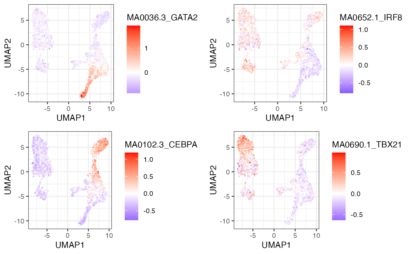
Gene activity
We can also define gene activity as the combined chromatin
accessibility of a gene promoter and peaks that correlated with it
across all accessibility profiles. This functionality is nicely
implemented in the cicero and monocle packages
and ChrAccR provides a wrapper function to compute gene
activities from DsATAC datasets:
# requires monocle3 to be installed
library(monocle3)

promoter_gr <- getCoord(dsa, "promoter")
names(promoter_gr) <- GenomicRanges::elementMetadata(promoter_gr)[,"gene_name"]
gene_act <- getCiceroGeneActivities(
  dsa,
  ".peaks.itlsi",
  promoterGr=promoter_gr,
  dimRedCoord=itlsi$pcaCoord
)
Analyzing the full dataset
The full dataset of the single-cell human hematopoiesis study (Granja et al.
2019) is publicly available. Here, we show how
ChrAccR can be applied to create a dataset from scratch
using the aligned fragment files as input. Downstream steps can be run
as shown above for the example subset of the data. Since the full
dataset comprises high-quality profiles for a large number of cells, the
analysis of such high-dimensional data has considerable resource
requirements. We recommend to run it on a machine with a large amount of
memory. The runtime for some of the folowing steps can exceed multiple
hours.
Preparing the input
The main input for creating a single-cell dataset in
ChrAccR are files containing the coordinates of sequenced
fragments. Such fragment files can be obtained from the output of the
CellRanger software (10x Genomics). For the hematopoiesis dataset
analyzed here (Granja et al. 2019), these files
are available from GEO (GEO
accession: GSE139369)). First, download the
GSE139369_RAW.tar file and unpack it (in the following, we
assume that you unpacked the files to a directory called
fragment_data). In addition to the fragment data, a sample
annotation table that contains information on the samples’ phenotypes
and technical parameters is needed. Here, we create one from the
filenames:
fragmentFiles <- list.files("fragment_data", pattern=".fragments.tsv.gz")
sampleAnnotation <- data.frame(
  sampleId = gsub("^(GSM[0-9]+)_scATAC_(.+).fragments\\.tsv\\.gz$", "\\2", fragmentFiles),
  geoAccession = gsub("^(GSM[0-9]+)_scATAC_(.+).fragments\\.tsv\\.gz$", "\\1", fragmentFiles),
  fragmentFilename = fragmentFiles,
  stringsAsFactors = FALSE
)
sampleAnnotation[,"source"] <- gsub("^(MPAL|CD34|BMMC|PBMC).+", "\\1", sampleAnnotation[,"sampleId"])
# only samples from healthy donors
sampleAnnotation <- sampleAnnotation[sampleAnnotation[,"source"]!="MPAL",]
inputFiles <- file.path('fragment_data', sampleAnnotation[,"fragmentFilename"])
Vanilla analysis
As demonstrated in the overview vignette, ChrAccR can
run a default analysis workflow by using the run_atac
function. For single-cell datasets, this requires you to supply a
reference to the fragment files or the output of the CellRanger
software, as well a sample annotation table:
setConfigElement("annotationColumns", c(".sampleId", "cellType", "nFrags", "tssEnrichment"))
dsa_full <- run_atac(config$.anaDir, input=inputFiles, sampleAnnot=sampleAnnotation, genome="hg19", sampleIdCol="sampleId")
Analysis steps in detail
Preparing the DsATAC data structure from fragment
files
Then we can directly create a DsATACsc dataset from the
fragment files:
dsa_full_raw <- DsATACsc.fragments(
  sampleAnnotation,
  inputFiles,
  "hg19",
  regionSets=NULL,
  sampleIdCol="sampleId",
  minFragsPerBarcode=1000L,
  maxFragsPerBarcode=50000L,
  keepInsertionInfo=TRUE
)
Filtering low quality cells
It is recommended to filter low quality cells from the datasets. In the code above, we already set a threshold for the minimum and maximum number of fragments for each cell in order for it to be included in the dataset. The following code also limits the dataset to cells that exhibit a sufficiently high signal-to-noise ratio, as defined by the enrichment of Tn5 insertions at transcription start sites (TSS) relative to background.
tsse_cutoff <- 8
dsa_full <- filterCellsTssEnrichment(dsa_full_raw, tsse_cutoff)
Dimension reduction and clustering using iterative LSI
We recommend to use the iterative LSI approach outlined above to obtain a relatively robust dimensionality reduction and clustering of cells. We compute the reduced components and coordinates in the code below. We also add the assigned cluster for each cell to the dataset annotation and aggregate the Tn5 insertion counts for the computed consensus peak set.
itlsi <- iterativeLSI(dsa_full, it0regionType="tiling5kb", it0clusterResolution=0.4, it1clusterResolution=0.4, it2clusterResolution=0.4)

# add cluster assignment to cell annotation
dsa_full <- addSampleAnnot(dsa_full, "cluster_itlsi", itlsi$clustAss)

# aggregate insertions accross the consensus set of cluster peaks derived during iterative LSI
dsa_full <- regionAggregation(dsa_full, itlsi$clusterPeaks_unfiltered, "peaks_itlsi", signal="insertions", dropEmpty=FALSE, bySample=FALSE)
Analysis reports
ChrAccR also provides methods to automatically generate
analysis reports that summarize most of the above analysis steps. The
reports for the full single-cell dataset described here can also be
found in the ‘Resource’
section of the ChrAccR website. Provided with a DsATAC
dataset these reports can be generated with a call to the corresponding
createReport_* function. For instance, the
createReport_summary generates a report containing an
overview of sample and cell statistics:
createReport_summary(dsa_full, file.path("reports"))The report generated by the createReport_exploratory
functions comprises unsupervised analysis, including dimensionality
reduction and the quantification of transcription factor activities.
Analysis parameters for generating these reports can be configures using
the setConfigElement function.
chromVarMotifsToPlot <- c("MA0036.3_GATA2", "MA0652.1_IRF8", "MA0102.3_CEBPA", "MA0466.2_CEBPB", "MA1141.1_FOS::JUND", "MA0080.4_SPI1", "MA0105.4_NFKB1", "MA0014.3_PAX5", "MA0002.2_RUNX1", "MA0690.1_TBX21")

setConfigElement("annotationColumns", c(".sampleId", "cellType", "nFrags", "tssEnrichment"))
setConfigElement("scIterativeLsiRegType", "tiling5kb")
setConfigElement("scIterativeLsiClusterResolution", 0.4)
setConfigElement("chromVarMotifNamesForDimRed", chromVarMotifsToPlot)

createReport_exploratory(dsa_full, file.path("reports"))
Session Info
Sys.Date()> [1] "2026-09-28"> R version 4.4.1 (2024-06-14)
> Platform: x86_64-conda-linux-gnu
> Running under: Debian GNU/Linux 12 (bookworm)
>
> Matrix products: default
> BLAS/LAPACK: /icbb/projects/share/software/packages/miniconda3/envs/ChrAccR/lib/libopenblasp-r0.3.29.so; LAPACK version 3.12.0
>
> locale:
> [1] C
>
> time zone: Europe/Berlin
> tzcode source: system (glibc)
>
> attached base packages:
> [1] stats graphics grDevices utils datasets methods base
>
> other attached packages:
> [1] ggplot2_3.5.2 ChrAccR_0.9.26
>
> loaded via a namespace (and not attached):
> [1] RColorBrewer_1.1-3 jsonlite_2.0.0
> [3] magrittr_2.0.3 farver_2.1.2
> [5] rmarkdown_2.29 fs_1.6.6
> [7] BiocIO_1.16.0 zlibbioc_1.52.0
> [9] ragg_1.4.0 vctrs_0.6.5
> [11] memoise_2.0.1 Rsamtools_2.22.0
> [13] RCurl_1.98-1.16 htmltools_0.5.8.1
> [15] S4Arrays_1.6.0 curl_6.2.2
> [17] Rhdf5lib_1.28.0 CNEr_1.42.0
> [19] SparseArray_1.6.0 rhdf5_2.50.0
> [21] sass_0.4.10 bslib_0.9.0
> [23] htmlwidgets_1.6.4 desc_1.4.3
> [25] plyr_1.8.9 plotly_4.10.4
> [27] cachem_1.1.0 GenomicAlignments_1.42.0
> [29] mime_0.13 lifecycle_1.0.4
> [31] pkgconfig_2.0.3 Matrix_1.7-3
> [33] R6_2.6.1 fastmap_1.2.0
> [35] GenomeInfoDbData_1.2.13 MatrixGenerics_1.18.0
> [37] shiny_1.10.0 digest_0.6.37
> [39] colorspace_2.1-1 TFMPvalue_0.0.9
> [41] AnnotationDbi_1.68.0 S4Vectors_0.44.0
> [43] textshaping_1.0.0 GenomicRanges_1.58.0
> [45] RSQLite_2.3.9 seqLogo_1.72.0
> [47] labeling_0.4.3 httr_1.4.7
> [49] abind_1.4-5 compiler_4.4.1
> [51] bit64_4.6.0-1 withr_3.0.2
> [53] BiocParallel_1.40.0 DBI_1.2.3
> [55] HDF5Array_1.34.0 R.utils_2.13.0
> [57] poweRlaw_1.0.0 DelayedArray_0.32.0
> [59] rjson_0.2.23 BSgenome.Hsapiens.UCSC.hg19_1.4.3
> [61] gtools_3.9.5 caTools_1.18.3
> [63] tools_4.4.1 httpuv_1.6.15
> [65] R.oo_1.27.0 glue_1.8.0
> [67] restfulr_0.0.15 rhdf5filters_1.18.0
> [69] promises_1.3.2 grid_4.4.1
> [71] reshape2_1.4.4 TFBSTools_1.44.0
> [73] generics_0.1.3 gtable_0.3.6
> [75] BSgenome_1.74.0 tzdb_0.5.0
> [77] R.methodsS3_1.8.2 nabor_0.5.0
> [79] tidyr_1.3.1 data.table_1.17.0
> [81] hms_1.1.3 XVector_0.46.0
> [83] BiocGenerics_0.52.0 RcppAnnoy_0.0.22
> [85] motifmatchr_1.28.0 pillar_1.10.2
> [87] stringr_1.5.1 later_1.4.2
> [89] muRtools_0.9.6 dplyr_1.1.4
> [91] lattice_0.22-7 rtracklayer_1.66.0
> [93] bit_4.6.0 chromVAR_1.28.0
> [95] annotate_1.84.0 tidyselect_1.2.1
> [97] DirichletMultinomial_1.48.0 GO.db_3.20.0
> [99] Biostrings_2.74.0 miniUI_0.1.2
> [101] knitr_1.50 IRanges_2.40.0
> [103] SummarizedExperiment_1.36.0 stats4_4.4.1
> [105] xfun_0.52 Biobase_2.66.0
> [107] matrixStats_1.5.0 DT_0.33
> [109] stringi_1.8.7 UCSC.utils_1.2.0
> [111] lazyeval_0.2.2 yaml_2.3.10
> [113] evaluate_1.0.3 codetools_0.2-20
> [115] ChrAccRex_0.3 tibble_3.2.1
> [117] cli_3.6.5 xtable_1.8-4
> [119] systemfonts_1.2.1 jquerylib_0.1.4
> [121] dichromat_2.0-0.1 Rcpp_1.0.14
> [123] GenomeInfoDb_1.42.0 png_0.1-8
> [125] XML_3.99-0.17 parallel_4.4.1
> [127] pkgdown_2.1.2 readr_2.1.5
> [129] blob_1.2.4 bitops_1.0-9
> [131] JASPAR2018_1.1.1 pwalign_1.2.0
> [133] viridisLite_0.4.2 muLogR_0.2
> [135] scales_1.4.0 purrr_1.0.4
> [137] crayon_1.5.3 rlang_1.1.6
> [139] cowplot_1.1.3 KEGGREST_1.46.0