Analysis of ATAC-seq
data
using ChrAccR
using ChrAccR
Fabian Mueller
2026-09-28
Source:vignettes/overview.Rmd
overview.Rmd
Introduction
ChrAccR is an R package that provides tools for the
comprehensive analysis chromatin accessibility data. The package
implements methods for data quality control, exploratory analyses
(including unsupervised methods for dimension reduction, clustering and
quantifying transcription factor activities) and the identification and
characterization of differentially accessible regions. It can be used
for the analysis of large bulk datasets comprising hundreds of samples
as well as for single-cell datasets with 10s to 100s of thousands of
cells.
Requiring only a limited set of R commands, ChrAccR
generates analysis reports that can be interactively explored,
facilitate a comprehensive analysis overview of a given dataset and are
easily shared with collaborators. The package is therefore particularly
useful for users with limited bioinformatic expertise, researchers new
to chromatin analysis or institutional core facilities providing
ATAC-seq as a service. Additionally, the package provides numerous
utility functions for custom R scripting that allow more in-depth
analyses of chromatin accessibility datasets.
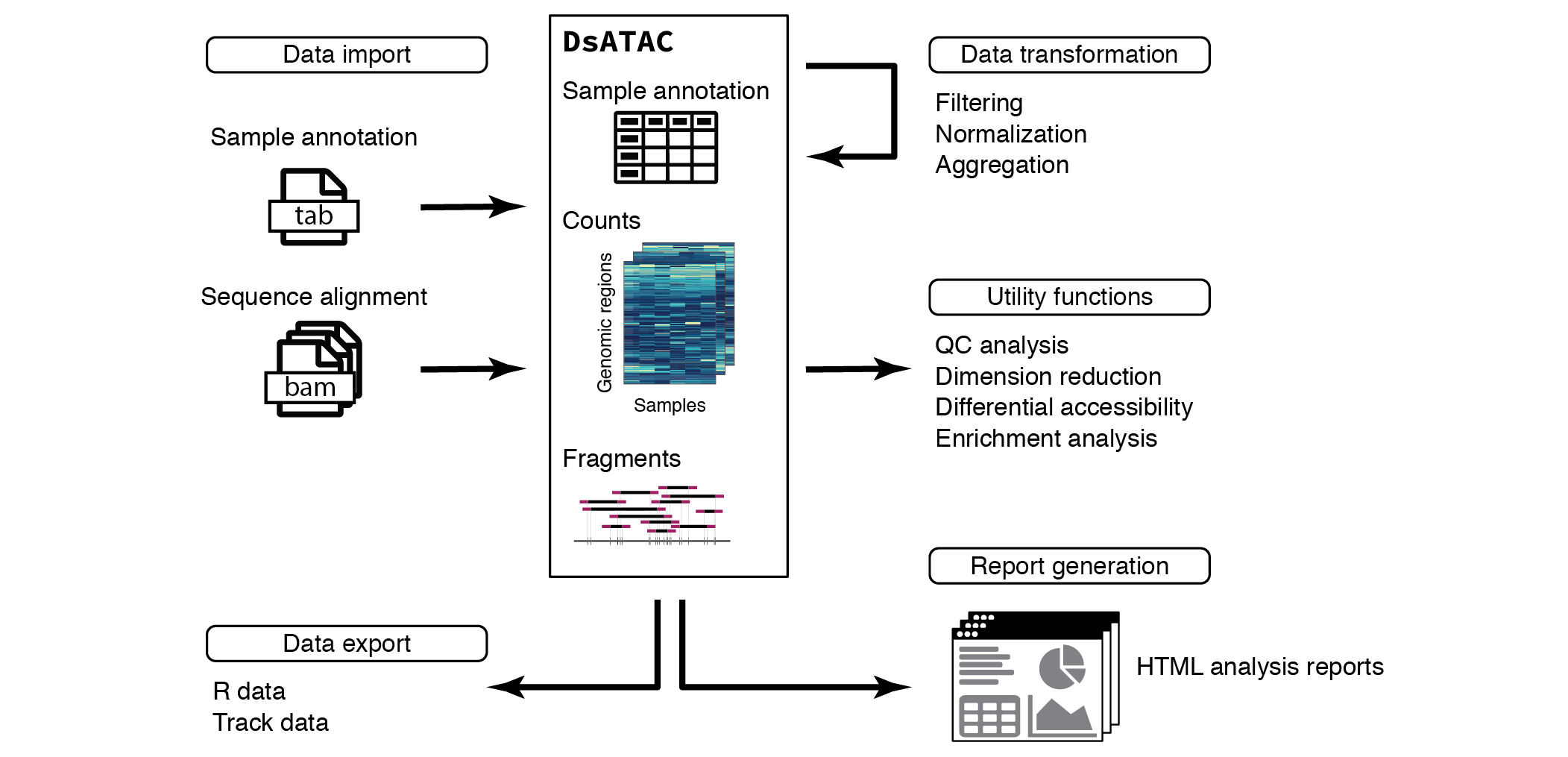
ChrAccR
This vignette focuses on the analysis of ATAC-seq data. This data can
be directly imported from aligned sequencing reads into a
DsATAC object, the main data structure for working with
ATAC-seq data. Using a small example dataset of chromatin accessibility
in human immune cells, this vignette covers filtering, normalizing and
aggregating count data across genomic regions of interest and introduces
convenient utility functions for quality control (QC), data exploration
and differential analysis. Additionally, ChrAccR
facilitates the automatic generation of analysis reports using several
preconfigured workflows.
We first provide instructions for running the entire analysis in a
‘’vanilla’’ workflow and then dive a little deeper into the underlying
data structures and custom analysis methods that ChrAccR
provides for highly individualized analyses.
Installation
To install ChrAccR and its dependencies, use the
devtools installation routine:
# install devtools if not previously installed
if (!is.element('devtools', installed.packages()[,"Package"])) install.packages('devtools')

# install dependencies
devtools::install_github("demuellae/muLogR")
devtools::install_github("demuellae/muRtools")
devtools::install_github("demuellae/muReportR")

# install ChrAccR
devtools::install_github("EpigenomeInformatics/ChrAccR", dependencies=TRUE)
We also provide complementary packages that contain genome-specific annotations. We highly recommend installing these annotation packages in order to speed up certain steps of the analysis:
# hg38 annotation package
install.packages("https://muellerf.s3.amazonaws.com/data/ChrAccR/data/annotation/ChrAccRAnnotationHg38_0.0.1.tar.gz")
Preparing the workspace
Loading ChrAccR works just like loading any other R
package
Example data
The ChrAccRex data package contains a small example
ATAC-seq datasets for ChrAccR. If you haven’t already
installed ChrAccRex use
devtools::install_github("EpigenomeInformatics/ChrAccRex")Note that many of the plots created in this vignette use the
excellent ggplot2 package. The following code loads the
package and sets a different plotting theme:
library(ggplot2)
# use a grid-less theme
theme_set(muRtools::theme_nogrid())
Vanilla analysis
We start by running the entire analysis pipeline on an example
dataset. After annotating the samples to be used in the analysis and
specifying a couple of analysis parameters, this can essentially be done
using just one command (run_atac(...)).
Example dataset
We provide an example dataset of ATAC-seq profiles of a subset of 33 human T cell samples taken from (Calderon et al. 2019). This dataset contains BAM files as well as a sample annotation table. If you have not already done so, please download and unzip the dataset:
# download and unzip the dataset
datasetUrl <- "https://s3.amazonaws.com/muellerf/data/ChrAccR/data/tutorial/tcells.zip"
downFn <- "tcells.zip"
download.file(datasetUrl, downFn)
unzip(downFn, exdir=".")
Configuring the analysis
A properly curated sample annotation table is essential for the entire analysis. Such an annotation at the minimum should contain sample identifiers, but ideally contains all sorts of available information for each sample, such as phenotypical and technical metadata. This especially includes information relevant for sample gouping and differential analysis. In the example dataset, we provide such an annotation table:
# prepare the sample annotation table
sampleAnnotFn <- file.path("tcells", "samples.tsv")
bamDir <- file.path("tcells", "bam")
sampleAnnot <- read.table(sampleAnnotFn, sep="\t", header=TRUE, stringsAsFactors=FALSE)
# add a column that ChrAccR can use to find the correct bam file for each sample
sampleAnnot[,"bamFilenameFull"] <- file.path(bamDir, sampleAnnot[,"bamFilename"])
Let us now also set a couple of analysis parameters and reporting
preferences. These options can be set using the
setConfigElement function and can be queried using
getConfigElement. A list of all available options is
contained in the documentation of setConfigElement
(e.g. use ?setConfigElement). Here, we tell ChrAccR which
annotation columns to focus on, which color schemes to use for some of
these annotation, set filtering thresholds for low-coverage regions, the
normalization method to be used and specify what comparisons to use for
differential analysis:
setConfigElement("annotationColumns", c("cellType", "stimulus", "donor"))
setConfigElement("colorSchemes", c(
  getConfigElement("colorSchemes"),
  list(
    "stimulus"=c("U"="royalblue", "S"="tomato"),
    "cellType"=c("TCD8naive"="purple3", "TCD8EM"="purple4", "TeffNaive"="seagreen3", "TeffMem"="seagreen4")
  )
))
setConfigElement("filteringCovgCount", 1L)
setConfigElement("filteringCovgReqSamples", 0.25)
setConfigElement("filteringSexChroms", TRUE)
setConfigElement("normalizationMethod", "quantile")
diffCompNames <- c(
  "TeffNaive_U vs TeffMem_U [sampleGroup]",
  "TCD8naive_U vs TCD8EM_U [sampleGroup]"
)
setConfigElement("differentialCompNames", diffCompNames)
ChrAccR uses sets of predefined genomic regions to
summarize count data. By default, this includes 200bp-tiling windows.
The following code generates a list of custom region sets that we can
optionally use in the analysis. Here, we use 500-bp tiling regions a
consensus set of ATAC-seq peaks that were identified in a large cancer
dataset (Corces et
al. 2018).
# Download an ATAC peak set from a Pan-cancer dataset [doi:10.1126/science.aav1898]
cancerPeaks <- read.table("https://api.gdc.cancer.gov/data/116ebba2-d284-485b-9121-faf73ce0a4ec", sep="\t", header=TRUE, comment.char="", quote="", stringsAsFactors=FALSE)
cancerPeaks <- GenomicRanges::GRanges(cancerPeaks[,"seqnames"], IRanges::IRanges(start=cancerPeaks[,"start"], end=cancerPeaks[,"end"], names=cancerPeaks[,"name"]))
cancerPeaks <- sort(cancerPeaks) # sort
# a list of custom region sets
regionSetList <- list(
  tiling500bp = muRtools::getTilingRegions("hg38", width=500L, onlyMainChrs=TRUE),
  cancerPeaks = cancerPeaks
)
Running the analysis
After these preparatory steps, we can run through the default
ChrAccR workflow with a single command using the
run_atac function. Supplied with the sample annotation
table and a reference to BAM files (or BED files containing fragments),
it will automatically run the entire pipeline including importing the
dataset, quality control analysis, filtering, count normalization,
exploratory analysis and (optionally) differential accessibility
analysis.
run_atac("ChrAccR_analysis", "bamFilenameFull", sampleAnnot, genome="hg38", sampleIdCol="sampleId", regionSets=regionSetList)Overview of ChrAccR data structures
ChrAccR implements data structures for the convenient
handling of chromatin accessibility data. Its main class is the
DsAcc which represents the prototype for more specialized
S4 classes for different types of accessibility protocols.
Here, we focus on ATAC-seq data and the corresponding data structure is
called DsATAC. The example data loaded above is such a
DsATAC object.
Each DsATAC object contains
- A sample annotation table
- Genomic coordinates for one ore more region sets, such as promoters, enhancers, acessibility peaks or genomic tiling windows
- Aggregate counts for each genomic region as quantification of accessibility
- Optionally, the coordinates of sequencing fragments/reads
For playing around with the ChrAccR datastructures, we
use a reduced version of the (Calderon et al. 2019) dataset
which focuses on only a subset of the human genome (approximately 1%).
It is provided in the ChrAccRex package and can be loaded
using:
dsa <- ChrAccRex::loadExample("dsAtac_ia_example")> 2026-09-28 23:07:24 2.0 STATUS STARTED Loading region count data from HDF5
> 2026-09-28 23:07:24 2.0 STATUS Region type: promoters_gc_protein_coding
> 2026-09-28 23:07:24 2.0 STATUS Region type: IA_prog_peaks
> 2026-09-28 23:07:24 2.1 STATUS Region type: t200
> 2026-09-28 23:07:24 2.1 STATUS Region type: t10k
> 2026-09-28 23:07:24 2.1 STATUS COMPLETED Loading region count data from HDF5
>
> 2026-09-28 23:07:24 2.1 STATUS STARTED Updating fragment RDS file references
> 2026-09-28 23:07:24 2.1 STATUS COMPLETED Updating fragment RDS file referencesTo get an overview of what information is stored in the example dataset, you can just type the object name:
dsa> DsATAC chromatin accessibility dataset
> [contains disk-backed data]
> contains:
> * 33 samples: TCD8EM_S_1001, TCD8EM_S_1002, TCD8EM_S_1003, TCD8EM_S_1004, TCD8EM_U_1001, ...
> * fragment data for 33 samples [disk-backed]
> * 4 region types: promoters_gc_protein_coding, IA_prog_peaks, t200, t10k
> * * 210 regions of type promoters_gc_protein_coding
> * * 13730 regions of type IA_prog_peaks
> * * 135004 regions of type t200
> * * 2704 regions of type t10kAccessing information in DsATAC datasets
Here are some utility functions that summarize the samples contained in the dataset:
# get the number of samples
length(dsa)
> [1] 33
# get the sample names
head(getSamples(dsa))
> [1] "TCD8EM_S_1001" "TCD8EM_S_1002" "TCD8EM_S_1003" "TCD8EM_S_1004"
> [5] "TCD8EM_U_1001" "TCD8EM_U_1002"
# sample annotation table
str(getSampleAnnot(dsa))
> 'data.frame': 33 obs. of 8 variables:
> $ sampleId : chr "TCD8EM_S_1001_a;TCD8EM_S_1001_b" "TCD8EM_S_1002_a;TCD8EM_S_1002_b" "TCD8EM_S_1003_a;TCD8EM_S_1003_b" "TCD8EM_S_1004_a;TCD8EM_S_1004_b" ...
> $ cellType : chr "TCD8EM" "TCD8EM" "TCD8EM" "TCD8EM" ...
> $ donor : chr "1001" "1002" "1003" "1004" ...
> $ stimulus : chr "S" "S" "S" "S" ...
> $ replicate : chr "a;b" "a;b" "a;b" "a;b" ...
> $ sampleGroup : chr "TCD8EM_S" "TCD8EM_S" "TCD8EM_S" "TCD8EM_S" ...
> $ replicateGroup: chr "TCD8EM_S_1001" "TCD8EM_S_1002" "TCD8EM_S_1003" "TCD8EM_S_1004" ...
> $ dataset : chr "ImmuneAtlas" "ImmuneAtlas" "ImmuneAtlas" "ImmuneAtlas" ...To obtain information on the region sets that are contained in the dataset, use:
# the names of the different region types
getRegionTypes(dsa)
> [1] "promoters_gc_protein_coding" "IA_prog_peaks"
> [3] "t200" "t10k"
# number of regions for a particular region type
getNRegions(dsa, "promoters_gc_protein_coding")
> [1] 210
# genomic coordinates of a particular region type
getCoord(dsa, "promoters_gc_protein_coding")
> GRanges object with 210 ranges and 23 metadata columns:
> seqnames ranges strand | gr.width source
> <Rle> <IRanges> <Rle> | <integer> <factor>
> ENSG00000204219.9 chr1 23424241-23426240 - | 43680 HAVANA
> ENSG00000088280.18 chr1 23484069-23486068 - | 56006 HAVANA
> ENSG00000007968.6 chr1 23530721-23532720 - | 24791 HAVANA
> ENSG00000117318.8 chr1 23559295-23561294 - | 1877 HAVANA
> ENSG00000197880.8 chr1 23579995-23581994 + | 59074 HAVANA
> ... ... ... ... . ... ...
> ENSG00000187026.2 chr21 30746734-30748733 - | 440 HAVANA
> ENSG00000187005.4 chr21 30754929-30756928 - | 599 HAVANA
> ENSG00000183640.5 chr21 30812753-30814752 - | 556 HAVANA
> ENSG00000274749.1 chr21 30829260-30831259 - | 721 HAVANA
> ENSG00000182591.5 chr21 30881056-30883055 - | 912 HAVANA
> type score phase ID
> <factor> <numeric> <integer> <character>
> ENSG00000204219.9 gene NA <NA> ENSG00000204219.9
> ENSG00000088280.18 gene NA <NA> ENSG00000088280.18
> ENSG00000007968.6 gene NA <NA> ENSG00000007968.6
> ENSG00000117318.8 gene NA <NA> ENSG00000117318.8
> ENSG00000197880.8 gene NA <NA> ENSG00000197880.8
> ... ... ... ... ...
> ENSG00000187026.2 gene NA <NA> ENSG00000187026.2
> ENSG00000187005.4 gene NA <NA> ENSG00000187005.4
> ENSG00000183640.5 gene NA <NA> ENSG00000183640.5
> ENSG00000274749.1 gene NA <NA> ENSG00000274749.1
> ENSG00000182591.5 gene NA <NA> ENSG00000182591.5
> gene_id gene_type gene_name level
> <character> <character> <character> <character>
> ENSG00000204219.9 ENSG00000204219.9 protein_coding TCEA3 2
> ENSG00000088280.18 ENSG00000088280.18 protein_coding ASAP3 1
> ENSG00000007968.6 ENSG00000007968.6 protein_coding E2F2 2
> ENSG00000117318.8 ENSG00000117318.8 protein_coding ID3 2
> ENSG00000197880.8 ENSG00000197880.8 protein_coding MDS2 2
> ... ... ... ... ...
> ENSG00000187026.2 ENSG00000187026.2 protein_coding KRTAP21-2 2
> ENSG00000187005.4 ENSG00000187005.4 protein_coding KRTAP21-1 2
> ENSG00000183640.5 ENSG00000183640.5 protein_coding KRTAP8-1 2
> ENSG00000274749.1 ENSG00000274749.1 protein_coding KRTAP7-1 2
> ENSG00000182591.5 ENSG00000182591.5 protein_coding KRTAP11-1 2
> havana_gene Parent transcript_id transcript_type
> <character> <list> <character> <character>
> ENSG00000204219.9 OTTHUMG00000003233.3 <NA> <NA>
> ENSG00000088280.18 OTTHUMG00000003234.7 <NA> <NA>
> ENSG00000007968.6 OTTHUMG00000003223.1 <NA> <NA>
> ENSG00000117318.8 OTTHUMG00000003229.2 <NA> <NA>
> ENSG00000197880.8 OTTHUMG00000002927.1 <NA> <NA>
> ... ... ... ... ...
> ENSG00000187026.2 OTTHUMG00000057769.2 <NA> <NA>
> ENSG00000187005.4 OTTHUMG00000057777.2 <NA> <NA>
> ENSG00000183640.5 OTTHUMG00000057771.1 <NA> <NA>
> ENSG00000274749.1 OTTHUMG00000188305.1 <NA> <NA>
> ENSG00000182591.5 OTTHUMG00000057773.1 <NA> <NA>
> transcript_name transcript_support_level tag
> <character> <character> <list>
> ENSG00000204219.9 <NA> <NA>
> ENSG00000088280.18 <NA> <NA>
> ENSG00000007968.6 <NA> <NA>
> ENSG00000117318.8 <NA> <NA>
> ENSG00000197880.8 <NA> <NA>
> ... ... ... ...
> ENSG00000187026.2 <NA> <NA>
> ENSG00000187005.4 <NA> <NA>
> ENSG00000183640.5 <NA> <NA>
> ENSG00000274749.1 <NA> <NA>
> ENSG00000182591.5 <NA> <NA>
> havana_transcript exon_number exon_id ont
> <character> <character> <character> <list>
> ENSG00000204219.9 <NA> <NA> <NA>
> ENSG00000088280.18 <NA> <NA> <NA>
> ENSG00000007968.6 <NA> <NA> <NA>
> ENSG00000117318.8 <NA> <NA> <NA>
> ENSG00000197880.8 <NA> <NA> <NA>
> ... ... ... ... ...
> ENSG00000187026.2 <NA> <NA> <NA>
> ENSG00000187005.4 <NA> <NA> <NA>
> ENSG00000183640.5 <NA> <NA> <NA>
> ENSG00000274749.1 <NA> <NA> <NA>
> ENSG00000182591.5 <NA> <NA> <NA>
> protein_id ccdsid
> <character> <character>
> ENSG00000204219.9 <NA> <NA>
> ENSG00000088280.18 <NA> <NA>
> ENSG00000007968.6 <NA> <NA>
> ENSG00000117318.8 <NA> <NA>
> ENSG00000197880.8 <NA> <NA>
> ... ... ...
> ENSG00000187026.2 <NA> <NA>
> ENSG00000187005.4 <NA> <NA>
> ENSG00000183640.5 <NA> <NA>
> ENSG00000274749.1 <NA> <NA>
> ENSG00000182591.5 <NA> <NA>
> -------
> seqinfo: 455 sequences from hg38 genomeYou can obtain a region-by-sample matrix containing Tn5 insertion
counts using the getCounts function:
>  num [1:210, 1:33] 99 527 288 339 29 381 355 364 231 613 ...
>  - attr(*, "dimnames")=List of 2
>   ..$ : NULL
>   ..$ : chr [1:33] "TCD8EM_S_1001" "TCD8EM_S_1002" "TCD8EM_S_1003" "TCD8EM_S_1004" ...
If the dataset contains fragment information, you can obtain the coordinates of sequencing fragments for each sample:
# number of fragments for the first 10 samples
getFragmentNum(dsa, sampleIds=getSamples(dsa)[1:10])
> TCD8EM_S_1001 TCD8EM_S_1002 TCD8EM_S_1003 TCD8EM_S_1004
> 330609 238663 164935 255774
> TCD8EM_U_1001 TCD8EM_U_1002 TCD8EM_U_1003 TCD8EM_U_1004
> 389454 263012 188389 286290
> TCD8naive_S_1001 TCD8naive_S_1002 TCD8naive_S_1003 TCD8naive_S_1004
> 279265 318357 182384 317368
> TCD8naive_U_1001 TCD8naive_U_1002 TCD8naive_U_1003 TCD8naive_U_1004
> 226051 331543 159358 473652
> TeffMem_S_1001 TeffMem_S_1002 TeffMem_S_1003 TeffMem_S_1004
> 229312 240847 126001 288532
> TeffMem_U_1001 TeffMem_U_1002 TeffMem_U_1003 TeffMem_U_1004
> 227925 281332 175000 225192
> TeffNaive_S_1001 TeffNaive_S_1002 TeffNaive_S_1003 TeffNaive_S_1004
> 305242 223408 132021 338461
> TeffNaive_S_1011 TeffNaive_U_1001 TeffNaive_U_1002 TeffNaive_U_1003
> 298524 159922 358213 177680
> TeffNaive_U_1004
> 347568
# start and end coordinates of all fragments for a given sample
getFragmentGr(dsa, "TCD8EM_U_1002")
> GRanges object with 263012 ranges and 1 metadata column:
> seqnames ranges strand | .sample
> <Rle> <IRanges> <Rle> | <character>
> [1] chr1 23400066-23400102 + | TCD8EM_U_1002_a
> [2] chr1 23400436-23400809 - | TCD8EM_U_1002_a
> [3] chr1 23403554-23403665 + | TCD8EM_U_1002_a
> [4] chr1 23403742-23404095 + | TCD8EM_U_1002_a
> [5] chr1 23403854-23404072 + | TCD8EM_U_1002_a
> ... ... ... ... . ...
> [263008] chr21 30999121-30999194 + | TCD8EM_U_1002_b
> [263009] chr21 30999121-30999196 + | TCD8EM_U_1002_b
> [263010] chr21 30999638-30999730 + | TCD8EM_U_1002_b
> [263011] chr21 30999758-30999969 - | TCD8EM_U_1002_b
> [263012] chr21 30999996-31000204 - | TCD8EM_U_1002_b
> -------
> seqinfo: 25 sequences from hg38 genome
# all Tn5 insertion sites (i.e. the concatenation of fragment start and end coordinates)
# for a set of samples
getInsertionSites(dsa, getSamples(dsa)[1:3])
> $TCD8EM_S_1001
> GRanges object with 661218 ranges and 1 metadata column:
> seqnames ranges strand | .sample
> <Rle> <IRanges> <Rle> | <character>
> [1] chr1 23399922 + | TCD8EM_S_1001_a
> [2] chr1 23399962 + | TCD8EM_S_1001_b
> [3] chr1 23400003 + | TCD8EM_S_1001_b
> [4] chr1 23400066 + | TCD8EM_S_1001_a
> [5] chr1 23400229 + | TCD8EM_S_1001_b
> ... ... ... ... . ...
> [661214] chr21 30999986 - | TCD8EM_S_1001_a
> [661215] chr21 30999995 - | TCD8EM_S_1001_a
> [661216] chr21 31000033 + | TCD8EM_S_1001_a
> [661217] chr21 31000038 - | TCD8EM_S_1001_b
> [661218] chr21 31000159 - | TCD8EM_S_1001_a
> -------
> seqinfo: 25 sequences from hg38 genome
>
> $TCD8EM_S_1002
> GRanges object with 477326 ranges and 1 metadata column:
> seqnames ranges strand | .sample
> <Rle> <IRanges> <Rle> | <character>
> [1] chr1 23399484 + | TCD8EM_S_1002_b
> [2] chr1 23400243 + | TCD8EM_S_1002_b
> [3] chr1 23400316 - | TCD8EM_S_1002_a
> [4] chr1 23400370 - | TCD8EM_S_1002_a
> [5] chr1 23400557 + | TCD8EM_S_1002_b
> ... ... ... ... . ...
> [477322] chr21 30999950 - | TCD8EM_S_1002_a
> [477323] chr21 30999993 + | TCD8EM_S_1002_b
> [477324] chr21 31000126 - | TCD8EM_S_1002_b
> [477325] chr21 31000157 + | TCD8EM_S_1002_a
> [477326] chr21 31000179 - | TCD8EM_S_1002_a
> -------
> seqinfo: 25 sequences from hg38 genome
>
> $TCD8EM_S_1003
> GRanges object with 329870 ranges and 1 metadata column:
> seqnames ranges strand | .sample
> <Rle> <IRanges> <Rle> | <character>
> [1] chr1 23400201 - | TCD8EM_S_1003_a
> [2] chr1 23400236 - | TCD8EM_S_1003_a
> [3] chr1 23400868 - | TCD8EM_S_1003_b
> [4] chr1 23400945 - | TCD8EM_S_1003_b
> [5] chr1 23401459 - | TCD8EM_S_1003_a
> ... ... ... ... . ...
> [329866] chr21 30998575 + | TCD8EM_S_1003_a
> [329867] chr21 30998962 + | TCD8EM_S_1003_a
> [329868] chr21 30999026 + | TCD8EM_S_1003_a
> [329869] chr21 30999928 + | TCD8EM_S_1003_a
> [329870] chr21 30999969 + | TCD8EM_S_1003_a
> -------
> seqinfo: 25 sequences from hg38 genomeManipulating DsATAC datasets
ChrAccR provides a number of functions for filtering a
dataset and for adding additional data.
Filtering for samples and genomic regions
For instance, if you want to work with only a subset of the data, you can remove samples and genomic regions from the dataset. The example contains data for resting (unstimulated) and stimulated T cells. The following code removes the stimulated cells and retains only the resting state cells:
isStim <- getSampleAnnot(dsa)[,"stimulus"] == "S"
dsa_resting <- removeSamples(dsa, isStim)
dsa_resting
> DsATAC chromatin accessibility dataset
> [contains disk-backed data]
> contains:
> * 16 samples: TCD8EM_U_1001, TCD8EM_U_1002, TCD8EM_U_1003, TCD8EM_U_1004, TCD8naive_U_1001, ...
> * fragment data for 16 samples [disk-backed]
> * 4 region types: promoters_gc_protein_coding, IA_prog_peaks, t200, t10k
> * * 210 regions of type promoters_gc_protein_coding
> * * 13730 regions of type IA_prog_peaks
> * * 135004 regions of type t200
> * * 2704 regions of type t10kSometimes you will want to focus on certain regions. For instance the following code filters the dataset, such that only the most variably accessible peaks are retained
peakCounts <- getCounts(dsa, "IA_prog_peaks")
# identify the 1000 most variable peaks
isVar <- rank(-matrixStats::rowVars(peakCounts)) <= 1000
# remove the less-variable peaks from the dataset
dsa_varPeaks <- removeRegions(dsa, !isVar, "IA_prog_peaks")
getNRegions(dsa_varPeaks, "IA_prog_peaks")
> [1] 1000There are also shortcuts for filtering certain regions from the dataset, for example:
# remove those regions that do not have at least 10 insertions in at least 75% of the samples
dsa_filtered <- filterLowCovg(dsa, thresh=10L, reqSamples=0.75)
> 2026-09-28 23:07:30 2.2 STATUS Removing regions with read counts lower than 10 in more than 8 samples (24%)
> 2026-09-28 23:07:30 2.2 INFO Removed 8 regions (3.81%) of type promoters_gc_protein_coding
> 2026-09-28 23:07:30 2.2 INFO Removed 11817 regions (86.07%) of type IA_prog_peaks
> 2026-09-28 23:07:30 2.3 INFO Removed 133034 regions (98.54%) of type t200
> 2026-09-28 23:07:30 2.3 INFO Removed 21 regions (0.78%) of type t10k
# remove regions on chromosome 21
dsa_filtered <- filterChroms(dsa, exclChrom=c("chr21"))
> 2026-09-28 23:07:30 2.3 INFO Removed 64 regions (30.48%) of type promoters_gc_protein_coding
> 2026-09-28 23:07:30 2.3 INFO Removed 7118 regions (51.84%) of type IA_prog_peaks
> 2026-09-28 23:07:30 2.3 INFO Removed 89001 regions (65.92%) of type t200
> 2026-09-28 23:07:30 2.3 INFO Removed 1781 regions (65.87%) of type t10k
> 2026-09-28 23:07:30 2.3 STATUS Filtering fragment dataTo remove a region type entirely, use
removeRegionType:
dsa_not10k <- removeRegionType(dsa, "t10k")
getRegionTypes(dsa_not10k)
> [1] "promoters_gc_protein_coding" "IA_prog_peaks"
> [3] "t200"Normalizing count data
ChrAccR provides several methods for normalizing and
adjusting the region count data. These methods can be accessed through
the transformCounts function:
# quantile normalization for all region types
dsa_qnorm <- transformCounts(dsa, method="quantile")
> 2026-09-28 23:07:37 2.2 STATUS STARTED Performing quantile normalization
> 2026-09-28 23:07:37 2.2 STATUS Region type: promoters_gc_protein_coding
> 2026-09-28 23:07:37 2.2 STATUS Region type: IA_prog_peaks
> 2026-09-28 23:07:37 2.2 STATUS Region type: t200
> 2026-09-28 23:07:42 2.3 STATUS Region type: t10k
> 2026-09-28 23:07:42 2.3 STATUS COMPLETED Performing quantile normalization
# RPKM normalization of peak counts
dsa_rpkm <- transformCounts(dsa, method="RPKM", regionTypes=c("IA_prog_peaks"))
> 2026-09-28 23:07:42 2.3 STATUS STARTED Performing RPKM normalization
> 2026-09-28 23:07:42 2.3 STATUS Region type: IA_prog_peaks
> 2026-09-28 23:07:42 2.3 STATUS COMPLETED Performing RPKM normalization
# log2(RPKM)
dsa_l2rpkm <- transformCounts(dsa_rpkm, method="log2", regionTypes=c("IA_prog_peaks"))
> 2026-09-28 23:07:42 2.3 STATUS STARTED log2 transforming counts
> 2026-09-28 23:07:42 2.3 STATUS Region type: IA_prog_peaks
> 2026-09-28 23:07:43 2.2 STATUS COMPLETED log2 transforming counts
# DESeq2 variance stabilizing transformation (vst)
dsa_vst <- transformCounts(dsa, method="vst", regionTypes=c("IA_prog_peaks"))
> 2026-09-28 23:07:43 2.2 STATUS STARTED Applying DESeq2 VST
> 2026-09-28 23:07:43 2.2 STATUS Region type: IA_prog_peaks> 2026-09-28 23:07:44 2.5 STATUS COMPLETED Applying DESeq2 VST
# correct for potential batch effects based on the annotated donor
dsa_vst <- transformCounts(dsa_vst, method="batchCorrect", batch=getSampleAnnot(dsa_qnorm)[,"donor"], regionTypes=c("IA_prog_peaks"))
> 2026-09-28 23:07:44 2.5 STATUS STARTED Applying batch effect correction
> 2026-09-28 23:07:44 2.5 STATUS Region type: IA_prog_peaks
> 2026-09-28 23:07:44 2.5 STATUS COMPLETED Applying batch effect correctionAdding a region type for count data aggregation
Sometimes you want to aggregate count data over a region set after
the DsATAC object has been created. Maybe you came up with
a better peak set or your collaborator provided you with a highly
interesting list of putative enhancer elements. These types of region
sets can be easily added to DsATAC objects using the
regionAggregation function. It is most useful, if the
dataset contains insertion/fragment data. The following example
downloads a set of putative regulatory elements defined by the Ensembl
Regulatory Build (Zerbino et al. 2015) of BLUEPRINT
epigenome data (http://www.blueprint-epigenome.eu/) and aggregates the
ATAC-seq insertions within these regions.
# download the file and prepare a GRanges object
regionFileUrl <- "http://medical-epigenomics.org/software/rnbeads/materials//data/regiondb/annotation_hg38_ensembleRegBuildBPall.RData"
downFn <- tempfile(pattern="regions", fileext="RData")
download.file(regionFileUrl, downFn)
regionEnv <- new.env()
load(downFn, envir=regionEnv)
regionGr <- unlist(regionEnv$regions)

# aggregate insertions across the new region type
dsa_erb <- regionAggregation(dsa, regionGr, "ERB", signal="insertions")
dsa_erb
Merging samples
You can also merge samples, e.g. from different technical or
biological replicates. In the following example, we merge all biological
replicates (originating from different donors) for the same cell type
and stimulation conditions. This grouping information is contained in
the sampleGroup annotation column. By default, counts will
be added up for each aggregated region, but you can specify other
aggregation methods such as the mean or median in the
countAggrFun argument.
dsa_merged <- mergeSamples(dsa, "sampleGroup", countAggrFun="sum")> 2026-09-28 23:07:44 2.5 STATUS Merging samples (region set: 'promoters_gc_protein_coding')...
> 2026-09-28 23:07:44 2.5 STATUS Merging samples (region set: 'IA_prog_peaks')...
> 2026-09-28 23:07:44 2.5 STATUS Merging samples (region set: 't200')...
> 2026-09-28 23:07:46 2.6 STATUS Merging samples (region set: 't10k')...
> 2026-09-28 23:07:46 2.6 STATUS STARTED Merging sample fragment data
> 2026-09-28 23:07:46 2.6 STATUS Merged sample 1 of 8
> 2026-09-28 23:07:47 2.6 STATUS Merged sample 2 of 8
> 2026-09-28 23:07:48 2.6 STATUS Merged sample 3 of 8
> 2026-09-28 23:07:49 2.6 STATUS Merged sample 4 of 8
> 2026-09-28 23:07:51 2.6 STATUS Merged sample 5 of 8
> 2026-09-28 23:07:52 2.6 STATUS Merged sample 6 of 8
> 2026-09-28 23:07:53 2.6 STATUS Merged sample 7 of 8
> 2026-09-28 23:07:54 2.6 STATUS Merged sample 8 of 8
> 2026-09-28 23:07:56 2.6 STATUS COMPLETED Merging sample fragment data
getSamples(dsa_merged)> [1] "TCD8EM_S" "TCD8EM_U" "TCD8naive_S" "TCD8naive_U" "TeffMem_S"
> [6] "TeffMem_U" "TeffNaive_S" "TeffNaive_U"Saving and loading datasets
In many analysis workflow, you want to save an R dataset to disk in
order to use it in downstream analysis using custom R scripts. Note that
R’s workflow of saveRDS readRDS is generally
not applicable for saving and loading DsATAC datasets,
because ChrAccR optionally uses disk-backed data structures
in order to be more memory efficient in the analysis. Instead, please
use ChrAccR’s functions:
> 2026-09-28 23:07:56     2.6  STATUS STARTED Saving region count data to HDF5
> 2026-09-28 23:07:56     2.6  STATUS     Region type: promoters_gc_protein_coding
> 2026-09-28 23:07:56     2.6  STATUS     Region type: IA_prog_peaks
> 2026-09-28 23:07:56     2.6  STATUS     Region type: t200
> 2026-09-28 23:07:58     2.5  STATUS     Region type: t10k
> 2026-09-28 23:07:58     2.5  STATUS COMPLETED Saving region count data to HDF5
>
> 2026-09-28 23:07:58     2.5  STATUS STARTED Saving fragment data to RDS
> 2026-09-28 23:07:58     2.5  STATUS COMPLETED Saving fragment data to RDS
dsa_reloaded <- loadDsAcc(dest)> 2026-09-28 23:07:58 2.5 STATUS STARTED Loading region count data from HDF5
> 2026-09-28 23:07:58 2.5 STATUS Region type: promoters_gc_protein_coding
> 2026-09-28 23:07:58 2.5 STATUS Region type: IA_prog_peaks
> 2026-09-28 23:07:58 2.5 STATUS Region type: t200
> 2026-09-28 23:07:58 2.5 STATUS Region type: t10k
> 2026-09-28 23:07:58 2.5 STATUS COMPLETED Loading region count data from HDF5
>
> 2026-09-28 23:07:58 2.5 STATUS STARTED Updating fragment RDS file references
> 2026-09-28 23:07:58 2.5 STATUS COMPLETED Updating fragment RDS file references
dsa_reloaded> DsATAC chromatin accessibility dataset
> [contains disk-backed data]
> contains:
> * 33 samples: TCD8EM_S_1001, TCD8EM_S_1002, TCD8EM_S_1003, TCD8EM_S_1004, TCD8EM_U_1001, ...
> * fragment data for 33 samples [disk-backed]
> * 4 region types: promoters_gc_protein_coding, IA_prog_peaks, t200, t10k
> * * 210 regions of type promoters_gc_protein_coding
> * * 13730 regions of type IA_prog_peaks
> * * 135004 regions of type t200
> * * 2704 regions of type t10kIf you ran the vanilla analysis using
`as described above, you automatically generated and savedDsATACdatasets. They are stored in thedatasubdirectory of your analysis directory (ChrAccR_analysis`):
Importing ATAC-seq data
Importing data from bam files
ATAC-seq data can be read from BAM files that contain aligned reads.
These reads originate from fragments whose endpoints resemble Tn5
insertion sites. All ChrAccR needs to read the input files
is a sample annotation table and pointers to the BAM files. The
following code reads the sample annotation table from the supplied text
file and adds a column that contains the BAM file locations on your disk
for each sample. Additionally, we prepare a list of region sets
(genome-wide tiling regions with window sizes of 500bp and 5kb) that we
want to aggregate the insertion counts over. Using the dataset
downloaded and prepared in the ‘Vanilla analysis’ section of this
vignette, we can easily create a DsATAC dataset using the
DsATAC.bam function. Supplied with the sample annotation
table and a reference to the BAM files, it will automatically determine
Tn5 insertion sites from the BAM files and aggregate counts over the
optionally supplied list of region sets (if no such list is provided,
200bp-tiling windows will be used as the default):
dsa_fromBam <- DsATAC.bam(sampleAnnot, "bamFilenameFull", "hg38", regionSets=regionSetList, sampleIdCol="sampleId")Analysis reports
ChrAccR provides a way to bundle certain types of
analyses into workflows that automatically create analysis reports.
These HTML-based analysis reports can be viewed in any web browser and
provide a convenient overview of the analysis results that can easily
shared with collaborators. ChrAccR provides the following
workflows:
-
summary: dataset characterization and quality control -
exploratory: exploratory analyses such as dimension reduction, clustering, TF motif enrichment, etc. -
differential: differential accessibility analysis between groups of samples
Provided with a DsATAC dataset, the workflows can be
started using the createReport_X() functions (where
X is the name of the workflow). Workflow options can be
specified using the setConfigElement() function for setting
ChrAccR’s options. Here are some option examples:
# exclude the promoter and 't10k' (10kb tiling windows) region types from the analysis
setConfigElement("regionTypes", setdiff(getRegionTypes(dsa), c("promoters_gc_protein_coding", "t10k")))
# see the current option setting
getConfigElement("regionTypes")
> [1] "IA_prog_peaks" "t200"
# use the following sample annotation columns for exploratory analyses
setConfigElement("annotationColumns", c("cellType", "donor", "stimulus"))
# add a custom color scheme for the 'stimulus' and 'cellType' annotation columns
setConfigElement("colorSchemes", c(
    getConfigElement("colorSchemes"),
    list(
        "stimulus"=c("U"="#7fbc41", "S"="#de77ae"),
        "cellType"=c("TCD8naive"="#9ecae1", "TCD8EM"="#08519c", "TeffNaive"="#016c59", "TeffMem"="#014636")
    )
))
To see which options are available use the help function for
setConfigElement
?setConfigElementThe createReport_X() take a DsATAC dataset
as input and write their results to a report directory. Not that this
directory can only contain one report for each analysis workflow and the
function will result in an error if the directory already contains a
report of that type.
Summary analysis
To get an overview of an ATAC-seq dataset use
createReport_summary(). The resulting report will contain a
summary of the sample annotation, genomic coverage by sequencing reads
and QC metrics such as a summary of the fragment size distribution and
enrichment of Tn5 insertions at transcription start sites (TSS
enrichment).
reportDir <- file.path(".", "ChrAccR_reports")
# create the report (takes ~10 min on the example dataset)
createReport_summary(dsa, reportDir)
Exploratory analysis
The exploratory analysis reports comprises unsupervised analysis
results, such as dimension reduction plots and sample clustering.
Additionally, TF motif activity for peak region sets (those region sets
that contain 'peak' in their name) is assessed using the
chromVAR package (Schep et al. 2017).
# create the report (takes ~1 min on the example dataset)
createReport_exploratory(dsa_qnorm, reportDir)
Differential analysis
The differential analysis workflow focuses on the pairwise comparison
between groups of samples. The resulting report contains summary tables
and plot for each comparison (e.g. volcano plots). Differentially
accessible regions are identified using DESeq2 and multiple
p-value and rank cutoffs.
# differential analysis option settings
setConfigElement("differentialColumns", c("stimulus", "cellType"))
# adjust for the donor annotation in the differential test
setConfigElement("differentialAdjColumns", c("donor"))
# create the report (takes ~18 min on the example dataset)
createReport_differential(dsa, reportDir)
Utility functions
Principal component plot
To quickly obtain a dimension reduction plot based on a specific set
of regions in a DsATAC dataset, you can use the
getDimRedCoords.X functions from the muRtools
package:
cm <- getCounts(dsa_qnorm, "IA_prog_peaks")
pcaCoord <- muRtools::getDimRedCoords.pca(t(cm))
muRtools::getDimRedPlot(pcaCoord, annot=getSampleAnnot(dsa_qnorm), colorCol="cellType", shapeCol="stimulus")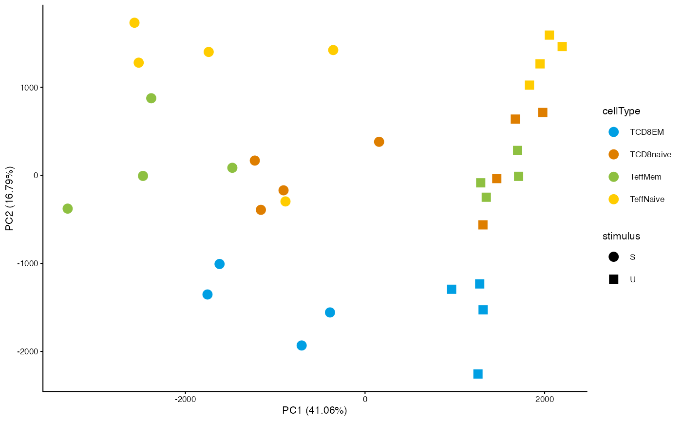
Plot the fragment size distribution
The fragment size distribution of an ATAC-seq can provide valuable quality control information. Typically, we expect a large number of fragments with sub-nucleosomal length (length < 200bp) and further peaks corresponding to 1,2, … nucleosomes (roughly multiples of 200bp in length). Here is how you can plot a corresponding density estimation of the fragment length distribution for a specific sample in the dataset.
plotInsertSizeDistribution(dsa, "TCD8EM_U_1002")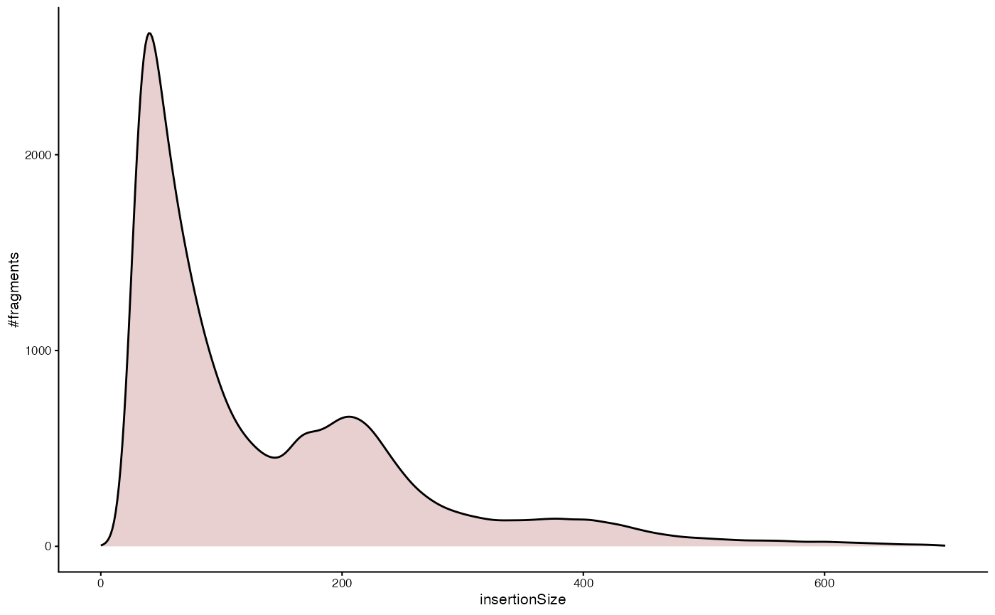
TSS enrichment plots
The enrichment of the number of fragments at transcription start
sites (TSS) over genomic background is a valuable indicator for the
signal-to-noise ratio in ATAC-seq data. In ChrAccR, the TSS
enrichment can be computed for each sample in a dataset using the
getTssEnrichment function. You will need the coordinates of
TSSs in the genome as input and the function will return an object
comprising a ggplot object as well as a numeric score that
quantifies the enrichment at the promoter (default definition: TSS +/-
2kb) vs a background (default: 100bp outside the promoter window).
Absolute and smoothed counts will be used for the computation.
# prepare a GRanges object of TSS coordinates
tssGr <- muRtools::getAnnotGrl.gencode("gencode.v27")[["gene"]]
tssGr <- tssGr[elementMetadata(tssGr)[,"gene_type"]=="protein_coding"]
tssGr <- promoters(tssGr, upstream=0, downstream=1)
tssGr

# compute TSS enrichment
tsse <- getTssEnrichment(dsa, "TCD8EM_U_1002", tssGr)
# enrichment score: number of insertions at the TSS
# over number of insertion in background regions
tsse$tssEnrichment
# plot
tsse$plot
Differential accessibility
daTab <- getDiffAcc(dsa, "IA_prog_peaks", "stimulus", grp1Name="S", grp2Name="U", adjustCols=c("cellType", "donor"))> 2026-09-28 23:08:00 2.6 WARNING The following design columns will not be considered because they do not have replicates: donorTranscription factor motif enrichment using
ChromVAR
Genome-wide aggregates across potential binding sites for
transcription factors can be extremely useful in the interpretation of
chromatin accessibility. The chromVAR package is designed
to quantify the overall TF motif accessibility for each sample in a
dataset (Schep et al.
2017). Using the getChromVarDev function, we can
obtain these deviation scores from DsATAC datasets:
cvRes <- getChromVarDev(dsa, "IA_prog_peaks", motifs="jaspar2018")
devZ <- chromVAR::deviationScores(cvRes)
str(devZ)
> num [1:452, 1:33] -1.0129 0.3066 -0.8639 -0.9216 -0.0197 ...
> - attr(*, "dimnames")=List of 2
> ..$ : chr [1:452] "MA0025.1_NFIL3" "MA0030.1_FOXF2" "MA0031.1_FOXD1" "MA0051.1_IRF2" ...
> ..$ : chr [1:33] "TCD8EM_S_1001" "TCD8EM_S_1002" "TCD8EM_S_1003" "TCD8EM_S_1004" ...
# plot a clustered heatmap of the first 20 motifs
pheatmap::pheatmap(devZ[1:20,])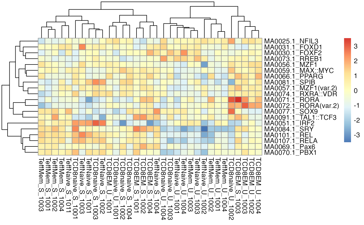
TF motif footprinting
To get an overview of the activity of certain transcription factors,
you can generate footprint plots which are aggreagtions of insertion
counts in windows surrounding all occurrences of a motif genome-wide.
ChrAccR normalizes these counts using kmer frequencies and also plots
the background distribution using all insertion sites (not just the ones
occurring near motifs). You can compute the data used to generate these
plots using the getMotifFootprints function. Note that
currently the computation of the kmer biases is quite compute intense.
We therefor recommend to limit the analysis to a few samples and
motifs.
motifNames <- c("MA1419.1_IRF4", "MA0139.1_CTCF", "MA0037.3_GATA3")
# motifNames <- grep("(IRF4|CTCF|GATA3)$", names(prepareMotifmatchr("hg38", "jaspar")$motifs), value=TRUE) # alternative by searching for patterns
samples <- c("TeffNaive_U_1001", "TeffNaive_U_1002", "TeffMem_U_1001", "TeffMem_U_1002")
fps <- getMotifFootprints(dsa, motifNames, samples)
# the results of the footprinting as data.frame for later plotting
str(fps[["MA0139.1_CTCF"]]$footprintDf)
# the result also contains a plot object, which can directly be drawn
fps[["MA0139.1_CTCF"]]$plot
Exporting to high-level Bioconductor data structures
ChrAccR offers utility functions to convert
accessibility data to other commonly used data structures for
Bioconductor-based workflows. For instance, to export count data
aggregated over a certain region type as a
SummarizedExperiments object you can use:
se <- getCountsSE(dsa, "IA_prog_peaks")
se
> class: RangedSummarizedExperiment
> dim: 13730 33
> metadata(0):
> assays(1): counts
> rownames: NULL
> rowData names(5): name score score_norm sampleId dataset
> colnames(33): TCD8EM_S_1001 TCD8EM_S_1002 ... TeffNaive_U_1003
> TeffNaive_U_1004
> colData names(8): sampleId cellType ... replicateGroup datasetTo export data as a DESeq2 dataset for differential
accessibility analysis:
dds <- getDESeq2Dataset(dsa, "IA_prog_peaks", designCols=c("donor", "stimulus", "cellType"))> 2026-09-28 23:08:38 3.1 WARNING The following design columns will not be considered because they do not have replicates: donor
dds> class: DESeqDataSet
> dim: 13730 33
> metadata(1): version
> assays(4): counts mu H cooks
> rownames: NULL
> rowData names(39): name score ... deviance maxCooks
> colnames(33): TCD8EM_S_1001 TCD8EM_S_1002 ... TeffNaive_U_1003
> TeffNaive_U_1004
> colData names(9): sampleId cellType ... dataset sizeFactorSession Info
Sys.Date()> [1] "2026-09-28"> R version 4.4.1 (2024-06-14)
> Platform: x86_64-conda-linux-gnu
> Running under: Debian GNU/Linux 12 (bookworm)
>
> Matrix products: default
> BLAS/LAPACK: /icbb/projects/share/software/packages/miniconda3/envs/ChrAccR/lib/libopenblasp-r0.3.29.so; LAPACK version 3.12.0
>
> locale:
> [1] C
>
> time zone: Europe/Berlin
> tzcode source: system (glibc)
>
> attached base packages:
> [1] stats graphics grDevices utils datasets methods base
>
> other attached packages:
> [1] ggplot2_3.5.2 ChrAccR_0.9.26
>
> loaded via a namespace (and not attached):
> [1] RColorBrewer_1.1-3 jsonlite_2.0.0
> [3] magrittr_2.0.3 farver_2.1.2
> [5] rmarkdown_2.29 fs_1.6.6
> [7] BiocIO_1.16.0 zlibbioc_1.52.0
> [9] ragg_1.4.0 vctrs_0.6.5
> [11] memoise_2.0.1 Rsamtools_2.22.0
> [13] RCurl_1.98-1.16 htmltools_0.5.8.1
> [15] S4Arrays_1.6.0 curl_6.2.2
> [17] Rhdf5lib_1.28.0 CNEr_1.42.0
> [19] SparseArray_1.6.0 rhdf5_2.50.0
> [21] sass_0.4.10 bslib_0.9.0
> [23] htmlwidgets_1.6.4 desc_1.4.3
> [25] plyr_1.8.9 plotly_4.10.4
> [27] cachem_1.1.0 GenomicAlignments_1.42.0
> [29] mime_0.13 lifecycle_1.0.4
> [31] pkgconfig_2.0.3 Matrix_1.7-3
> [33] R6_2.6.1 fastmap_1.2.0
> [35] GenomeInfoDbData_1.2.13 MatrixGenerics_1.18.0
> [37] shiny_1.10.0 digest_0.6.37
> [39] colorspace_2.1-1 TFMPvalue_0.0.9
> [41] AnnotationDbi_1.68.0 S4Vectors_0.44.0
> [43] DESeq2_1.46.0 textshaping_1.0.0
> [45] GenomicRanges_1.58.0 RSQLite_2.3.9
> [47] seqLogo_1.72.0 labeling_0.4.3
> [49] httr_1.4.7 abind_1.4-5
> [51] compiler_4.4.1 bit64_4.6.0-1
> [53] withr_3.0.2 BiocParallel_1.40.0
> [55] DBI_1.2.3 R.utils_2.13.0
> [57] HDF5Array_1.34.0 poweRlaw_1.0.0
> [59] DelayedArray_0.32.0 rjson_0.2.23
> [61] gtools_3.9.5 caTools_1.18.3
> [63] tools_4.4.1 httpuv_1.6.15
> [65] R.oo_1.27.0 glue_1.8.0
> [67] restfulr_0.0.15 rhdf5filters_1.18.0
> [69] promises_1.3.2 grid_4.4.1
> [71] reshape2_1.4.4 TFBSTools_1.44.0
> [73] generics_0.1.3 gtable_0.3.6
> [75] BSgenome_1.74.0 tzdb_0.5.0
> [77] R.methodsS3_1.8.2 preprocessCore_1.75.0
> [79] nabor_0.5.0 tidyr_1.3.1
> [81] data.table_1.17.0 hms_1.1.3
> [83] XVector_0.46.0 BiocGenerics_0.52.0
> [85] motifmatchr_1.28.0 pillar_1.10.2
> [87] stringr_1.5.1 limma_3.62.2
> [89] later_1.4.2 muRtools_0.9.6
> [91] dplyr_1.1.4 lattice_0.22-7
> [93] rtracklayer_1.66.0 bit_4.6.0
> [95] chromVAR_1.28.0 annotate_1.84.0
> [97] tidyselect_1.2.1 BSgenome.Hsapiens.UCSC.hg38_1.4.5
> [99] DirichletMultinomial_1.48.0 GO.db_3.20.0
> [101] locfit_1.5-9.12 Biostrings_2.74.0
> [103] miniUI_0.1.2 knitr_1.50
> [105] IRanges_2.40.0 SummarizedExperiment_1.36.0
> [107] stats4_4.4.1 xfun_0.52
> [109] Biobase_2.66.0 statmod_1.5.2
> [111] matrixStats_1.5.0 pheatmap_1.0.13
> [113] DT_0.33 stringi_1.8.7
> [115] UCSC.utils_1.2.0 lazyeval_0.2.2
> [117] yaml_2.3.10 evaluate_1.0.3
> [119] codetools_0.2-20 ChrAccRex_0.3
> [121] tibble_3.2.1 cli_3.6.5
> [123] xtable_1.8-4 systemfonts_1.2.1
> [125] jquerylib_0.1.4 dichromat_2.0-0.1
> [127] Rcpp_1.0.14 GenomeInfoDb_1.42.0
> [129] png_0.1-8 XML_3.99-0.17
> [131] parallel_4.4.1 pkgdown_2.1.2
> [133] readr_2.1.5 blob_1.2.4
> [135] bitops_1.0-9 JASPAR2018_1.1.1
> [137] pwalign_1.2.0 viridisLite_0.4.2
> [139] muLogR_0.2 scales_1.4.0
> [141] purrr_1.0.4 crayon_1.5.3
> [143] rlang_1.1.6 KEGGREST_1.46.0