A worked example with the ChrAccR example data

The data

ChrAccRex ships an ATAC-seq example dataset of sorted immune cells, aligned to hg38 and stored as a DsATAC object with fragment level data. That is what chromTFR needs: footprints are built from single base Tn5 cut positions, which only fragments provide.

remotes::install_github("EpigenomeInformatics/ChrAccRex")

library(chromTFR)
#> Loading required package: data.table
#> Loading required package: SummarizedExperiment
#> Loading required package: MatrixGenerics
#> Loading required package: matrixStats
#> 
#> Attaching package: 'MatrixGenerics'
#> The following objects are masked from 'package:matrixStats':
#> 
#>     colAlls, colAnyNAs, colAnys, colAvgsPerRowSet, colCollapse,
#>     colCounts, colCummaxs, colCummins, colCumprods, colCumsums,
#>     colDiffs, colIQRDiffs, colIQRs, colLogSumExps, colMadDiffs,
#>     colMads, colMaxs, colMeans2, colMedians, colMins, colOrderStats,
#>     colProds, colQuantiles, colRanges, colRanks, colSdDiffs, colSds,
#>     colSums2, colTabulates, colVarDiffs, colVars, colWeightedMads,
#>     colWeightedMeans, colWeightedMedians, colWeightedSds,
#>     colWeightedVars, rowAlls, rowAnyNAs, rowAnys, rowAvgsPerColSet,
#>     rowCollapse, rowCounts, rowCummaxs, rowCummins, rowCumprods,
#>     rowCumsums, rowDiffs, rowIQRDiffs, rowIQRs, rowLogSumExps,
#>     rowMadDiffs, rowMads, rowMaxs, rowMeans2, rowMedians, rowMins,
#>     rowOrderStats, rowProds, rowQuantiles, rowRanges, rowRanks,
#>     rowSdDiffs, rowSds, rowSums2, rowTabulates, rowVarDiffs, rowVars,
#>     rowWeightedMads, rowWeightedMeans, rowWeightedMedians,
#>     rowWeightedSds, rowWeightedVars
#> Loading required package: GenomicRanges
#> Loading required package: stats4
#> Loading required package: BiocGenerics
#> 
#> Attaching package: 'BiocGenerics'
#> The following objects are masked from 'package:stats':
#> 
#>     IQR, mad, sd, var, xtabs
#> The following objects are masked from 'package:base':
#> 
#>     Filter, Find, Map, Position, Reduce, anyDuplicated, aperm, append,
#>     as.data.frame, basename, cbind, colnames, dirname, do.call,
#>     duplicated, eval, evalq, get, grep, grepl, intersect, is.unsorted,
#>     lapply, mapply, match, mget, order, paste, pmax, pmax.int, pmin,
#>     pmin.int, rank, rbind, rownames, sapply, setdiff, sort, table,
#>     tapply, union, unique, unsplit, which.max, which.min
#> Loading required package: S4Vectors
#> 
#> Attaching package: 'S4Vectors'
#> The following objects are masked from 'package:data.table':
#> 
#>     first, second
#> The following object is masked from 'package:utils':
#> 
#>     findMatches
#> The following objects are masked from 'package:base':
#> 
#>     I, expand.grid, unname
#> Loading required package: IRanges
#> 
#> Attaching package: 'IRanges'
#> The following object is masked from 'package:data.table':
#> 
#>     shift
#> Loading required package: GenomeInfoDb
#> Loading required package: Biobase
#> Welcome to Bioconductor
#> 
#>     Vignettes contain introductory material; view with
#>     'browseVignettes()'. To cite Bioconductor, see
#>     'citation("Biobase")', and for packages 'citation("pkgname")'.
#> 
#> Attaching package: 'Biobase'
#> The following object is masked from 'package:MatrixGenerics':
#> 
#>     rowMedians
#> The following objects are masked from 'package:matrixStats':
#> 
#>     anyMissing, rowMedians
library(data.table)
library(ggplot2)
library(BSgenome.Hsapiens.UCSC.hg38)
#> Loading required package: BSgenome
#> Loading required package: Biostrings
#> Loading required package: XVector
#> 
#> Attaching package: 'Biostrings'
#> The following object is masked from 'package:base':
#> 
#>     strsplit
#> Loading required package: BiocIO
#> Loading required package: rtracklayer
#> 
#> Attaching package: 'rtracklayer'
#> The following object is masked from 'package:BiocIO':
#> 
#>     FileForFormat

dsa <- ChrAccRex::loadExample("dsAtac_ia_example")
#> 2026-09-28 23:06:35     2.1  STATUS STARTED Loading region count data from HDF5
#> 2026-09-28 23:06:35     2.1  STATUS     Region type: promoters_gc_protein_coding
#> 2026-09-28 23:06:35     2.1  STATUS     Region type: IA_prog_peaks
#> 2026-09-28 23:06:35     2.1  STATUS     Region type: t200
#> 2026-09-28 23:06:35     2.1  STATUS     Region type: t10k
#> 2026-09-28 23:06:35     2.1  STATUS COMPLETED Loading region count data from HDF5
#> 
#> 2026-09-28 23:06:35     2.1  STATUS STARTED Updating fragment RDS file references
#> 2026-09-28 23:06:35     2.1  STATUS COMPLETED Updating fragment RDS file references
ann <- getAccSampleAnnotation(dsa)
# The annotation is in the order of the samples, but its sampleId column
# lists the merged replicates, so take the ids from the object itself
ann$sample <- getAccSamples(dsa)
table(ann$cellType)
#> 
#>    TCD8EM TCD8naive   TeffMem TeffNaive 
#>         8         8         8         9
ChrAccR::getRegionTypes(dsa)
#> [1] "promoters_gc_protein_coding" "IA_prog_peaks"              
#> [3] "t200"                        "t10k"

This vignette compares naive against effector memory CD8 T cells, using three unstimulated samples of each. Restricting to a handful of samples keeps the build short; a real run would use all of them.

groups <- c("TCD8naive", "TCD8EM")
picked <- do.call(rbind, lapply(groups, function(g) {
    rows <- ann[ann$cellType == g & ann$stimulus == "U", , drop = FALSE]
    head(rows, 3)
}))
if (!all(groups %in% picked$cellType)) {
    stop("No unstimulated samples for: ",
        paste(setdiff(groups, picked$cellType), collapse = ", ")
    )
}
picked$sample
#> [1] "TCD8naive_U_1001" "TCD8naive_U_1002" "TCD8naive_U_1003" "TCD8EM_U_1001"   
#> [5] "TCD8EM_U_1002"    "TCD8EM_U_1003"

Insertion sites

The peaks of the example dataset are extended so that they still cover the flanks of a motif window, and the insertions are counted per base inside them. Scores are insertions per million, so samples of different depth stay comparable.

peaks <- getAccRegions(dsa, regionType = "IA_prog_peaks", extend = 500)

cache <- tempfile("chromTFR_example")
dir.create(cache)
files <- vapply(picked$sample, function(s) {
    f <- file.path(cache, paste0("ins_", s, ".RDS"))
    saveRDS(getTn5Insertions(dsa, s, regions = peaks), f)
    f
}, character(1))
#> INFO [2026-09-28 23:06:36] TCD8naive_U_1001: 452102 insertions, 260301 positions
#> INFO [2026-09-28 23:06:37] TCD8naive_U_1002: 663086 insertions, 392195 positions
#> INFO [2026-09-28 23:06:38] TCD8naive_U_1003: 318716 insertions, 205502 positions
#> INFO [2026-09-28 23:06:39] TCD8EM_U_1001: 778908 insertions, 395991 positions
#> INFO [2026-09-28 23:06:39] TCD8EM_U_1002: 526024 insertions, 266680 positions
#> INFO [2026-09-28 23:06:39] TCD8EM_U_1003: 376778 insertions, 203893 positions

mergeInsertionSites() pools the samples of a group into one aggregate, averaging the scores so that groups of unequal size stay on the same scale.

ins <- lapply(groups, function(g) {
    mergeInsertionSites(files[picked$cellType == g])
})
names(ins) <- groups
ins[["TCD8naive"]]
#> GRanges object with 775869 ranges and 2 metadata columns:
#>            seqnames    ranges strand |     score  coverage
#>               <Rle> <IRanges>  <Rle> | <numeric> <integer>
#>        [1]     chr1  23401088      * |  1.045863         1
#>        [2]     chr1  23401103      * |  0.737297         1
#>        [3]     chr1  23401106      * |  1.045863         1
#>        [4]     chr1  23401115      * |  0.502700         1
#>        [5]     chr1  23401122      * |  0.737297         1
#>        ...      ...       ...    ... .       ...       ...
#>   [775865]    chr21  31000002      * |  0.502700         1
#>   [775866]    chr21  31000017      * |  0.737297         1
#>   [775867]    chr21  31000054      * |  0.502700         1
#>   [775868]    chr21  31000171      * |  1.005400         2
#>   [775869]    chr21  31000448      * |  0.737297         1
#>   -------
#>   seqinfo: 4 sequences from an unspecified genome; no seqlengths

Binding sites

The annotation comes from methylTFRAnnotationHg38, unchanged from methylTFR. prepareTFBS() resizes the binding sites to the footprint window; everything downstream works on that object.

motifs <- c("CTCF", "FOS::JUN")
tf_bindsites <- methylTFRAnnotationHg38::getTFbindsites(
    motifSet = "jaspar2020"
)

tfbs <- lapply(motifs, function(m) prepareTFBS(tf_bindsites[[m]]))
names(tfbs) <- motifs
lengths(tfbs)
#>     CTCF FOS::JUN 
#>   554572   244961

The Tn5 k-mer model

Tn5 prefers some short sequences over others, and a motif is a fixed string of letters in the centre of every window, so part of any dip is chemistry rather than protein. The expected profile here measures that preference from the cuts themselves.

kmerBackground() counts every 6-mer of the accessible genome. It depends on the regions only, so it is computed once and reused for both groups.

genome <- BSgenome.Hsapiens.UCSC.hg38
kmer <- 6L
bg <- kmerBackground(peaks, genome, k = kmer)
#> INFO [2026-09-28 23:06:59] Counting background k-mers in 13730 regions

computeKmerBias() compares the 6-mer at each observed cut with that background. A weight above one means Tn5 cuts that word more often than its abundance predicts.

bias <- lapply(ins, computeKmerBias,
    regions = peaks, genome = genome, k = kmer, bg = bg, max.ins = 5e5
)
#> INFO [2026-09-28 23:07:00] Counting k-mers at 500000 insertion sites
#> INFO [2026-09-28 23:07:03] k-mer weights from 0.05 to 8.17
#> INFO [2026-09-28 23:07:03] Counting k-mers at 500000 insertion sites
#> INFO [2026-09-28 23:07:05] k-mer weights from 0.03 to 19.94
summary(bias[["TCD8naive"]])
#>    Min. 1st Qu.  Median    Mean 3rd Qu.    Max. 
#> 0.04925 0.70813 1.07103 1.29502 1.57287 8.17297

kmerBiasProfile() walks along the binding sites, reads the genomic 6-mer at each position and averages its weight across sites. That curve is what the insertions would look like with no protein bound.

expected <- lapply(groups, function(g) {
    prof <- lapply(motifs, function(m) {
        kmerBiasProfile(tfbs[[m]], genome, bias[[g]],
            k = kmer, max.sites = 5000
        )
    })
    names(prof) <- motifs
    prof
})
#> INFO [2026-09-28 23:07:43] Bias profile over 5000 sites
#> INFO [2026-09-28 23:08:02] Bias profile over 5000 sites
#> INFO [2026-09-28 23:08:11] Bias profile over 5000 sites
#> INFO [2026-09-28 23:08:17] Bias profile over 5000 sites
names(expected) <- groups

Footprints

accFootprintData() stacks the insertions on the centre of every binding site and matches the expected curve to the observed flanks.

profiles <- lapply(motifs, function(m) {
    e <- lapply(groups, function(g) expected[[g]][[m]])
    names(e) <- groups
    accFootprintData(tfbs[[m]], ins, e)
})
names(profiles) <- motifs
head(profiles[["CTCF"]])
#>        x      avg_ins     type     group
#>    <num>        <num>   <char>    <fctr>
#> 1:  -272 0.0003567070 Observed TCD8naive
#> 2:  -271 0.0003552325 Observed TCD8naive
#> 3:  -270 0.0003511040 Observed TCD8naive
#> 4:  -269 0.0003618358 Observed TCD8naive
#> 5:  -268 0.0003618812 Observed TCD8naive
#> 6:  -267 0.0003682324 Observed TCD8naive

The deviation score reads that curve as one number, the insertion density of the central window over the density of the outer flanks, minus the same ratio on the expected curve. A value below zero means the centre is more protected than the sequence alone predicts.

vapply(profiles, function(df) {
    df[group == "TCD8naive", accDeviation(.SD),
        .SDcols = c("x", "avg_ins", "type")]
}, numeric(1))
#>      CTCF  FOS::JUN 
#> 0.1659338 0.4797729

colours <- c(TCD8naive = "#3B6EA5", TCD8EM = "#B23A48")
plotAccFootprintGrid(profiles, tfbs, colours,
    corrected = "k-mer corrected"
)
#> INFO [2026-09-28 23:08:17] CTCF, k-mer corrected deviations: TCD8naive = 0.166, TCD8EM = 0.153
#> INFO [2026-09-28 23:08:17] FOS::JUN, k-mer corrected deviations: TCD8naive = 0.48, TCD8EM = 1.374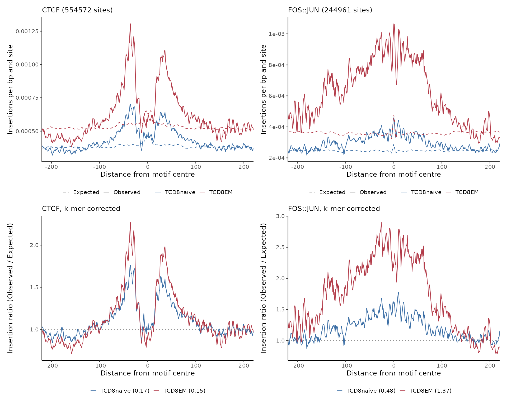

CTCF is the control to look at first: it binds stably, so its footprint is deep and the corrected curve dips well below one. AP-1 is the opposite case, a factor with a short residence time whose footprint stays shallow even where it is active.

A GC based expected profile is available as well, through addGCBintoAccessome() and computeAccExpectations(), and needs no genome sequence. Comparing the two on the same motif is a useful check: a dip that survives the k-mer correction is a footprint, one that flattens was Tn5 preferring the flanking sequence.

Session info