| Allele-specific chromatin accessibility | using ChrAccR • ChrAccR

Introduction

Both alleles of a heterozygous site sit in the same nucleus, see the same transcription factors and go through the same library preparation. Any difference in read counts between them comes from the sequence. That is what makes allele-specific chromatin accessibility (ASC) an internally controlled measurement: the second allele is the control.

AlleleSpeC is the ASC layer of ChrAccR. It takes WASP-corrected BAM files and donor genotypes, counts reference and alternative reads at heterozygous sites inside consensus peaks, tests each site for imbalance, and checks whether the imbalance follows the allele a transcription factor is predicted to bind. DsASC holds the data. It is a DsAcc subclass with two aligned count matrices (ref and alt, sites x samples) and the allele-agnostic peak matrix in the same object.

This vignette covers the pipeline end to end. The stages that need a cluster are shown but not run. Everything after counting runs on a small example object in inst/extdata, built by inst/scripts/make_vignette_data.R.

The shape of the pipeline

Stage	Runs in	Entry point	Produces
Genotyping	shell (GATK)	`01_call_variants.sh`	`{donor}_heterozygous.vcf.gz`
Mapping-bias correction	shell (WASP)	`03_wasp.R`	`{sample}_wasp.bam`
Shared site list	R	`buildMasterSNPs()`	master `GRanges` with donor membership
Allele counting	R	`DsASC.gatk()`	one `DsASC` per cell type
Peak restriction	R	`annotateASCSites()`, `filterASCByPeaks()`, `setAccessibility()`	`DsASC` limited to open chromatin
Genotype and bias cleanup	R	`ascDropHomozygous()`, `ascFilterRegions()`, `ascPoolReplicates()`	cleaned count matrices
Imbalance testing	R	`calcASCStatistics()`, `filterForRecurrence()`	per site-sample statistics
Cross-cell-type sharing	R	`ascAggregate()`, `ascSharing()`, `estimateSharedImbalance()`	sharing estimates
Motif disruption	R	`motifmatchr` scoring	per-site PWM delta table
Binding preference	R	per-site PWM preference bins	reference fraction by predicted preference, per condition

Genotyping and WASP are the slow steps, and they are also the ones that decide whether the results mean anything. The R functions below assume both were done properly.

Requirements

The ASC layer needs a few packages beyond the standard ChrAccR dependencies. VariantAnnotation and Rsamtools for reading genotypes and running the pileup, HDF5Array and DelayedArray for disk-backed counting, ashr for the sharing estimate, and JASPAR2020, TFBSTools, motifmatchr plus a BSgenome package for the motif step.

BiocManager::install(c("VariantAnnotation", "Rsamtools", "HDF5Array", "DelayedArray",
                       "JASPAR2020", "TFBSTools", "motifmatchr",
                       "BSgenome.Hsapiens.UCSC.hg38"))
install.packages("ashr")

library(ChrAccR)
library(GenomicRanges)
library(data.table)
library(ggplot2)
theme_set(theme_bw(base_size = 11))

Before R: genotypes and bias correction

Two things have to be right before any allele is counted. Neither can be repaired downstream.

The heterozygous sites have to be really heterozygous. Genotypes are called per donor, jointly across all of that donor’s libraries, so a call rests on the donor’s full depth instead of one shallow sample. Only biallelic SNVs called heterozygous are kept, one file per donor.

And reads carrying the alternative allele have to survive alignment. A read that differs from the reference maps slightly worse than one that matches, which pushes every site toward the reference allele and manufactures ASC out of nothing. WASP re-maps each overlapping read with its alleles swapped and throws away any read that does not come back to the same position.

Neither step runs from ChrAccR. You need to run the genotyping and WASP scripts first. They live in the AlleleSpeC repository at https://github.com/EpigenomeInformatics/allele_spec, together with an audit script that checks whether the correction actually worked.

Run that audit even when WASP reports success. It measures the pooled reference fraction per sample at that donor’s heterozygous sites. A corrected library sits near 0.5; anything above roughly 0.55 is still biased and will contaminate everything downstream.

The sample annotation needs sampleId, bamFilename and donor at minimum, plus cellType and stimulus for grouping and contrasts. Row names have to be the sample identifiers.

meta <- fread("tables/sampleAnnot_filtered.csv")
meta[, donor := as.character(donor)]
meta[, bamFilename := file.path(waspDir, paste0(sampleId, "_wasp.bam"))]
meta <- meta[file.exists(bamFilename)]

One site list for every donor

Donors do not share heterozygous sites, so counting each cell type against its own list gives objects whose rows do not line up. buildMasterSNPs() reads every donor VCF once and returns the sorted union of biallelic heterozygous SNPs, with a donorMembership column recording which donors are heterozygous at each site.

masterGr <- buildMasterSNPs(donors = unique(meta$donor), vcfDir = vcfDir, genome = "hg38")
saveRDS(masterGr, file.path(ascDir, "masterSNPs.rds"))

Build it once and reuse it. Row alignment is what makes it possible to ask later whether a site imbalanced in T cells is also imbalanced in B cells. The membership column lets each sample be counted only where its own donor is heterozygous and marked missing everywhere else.

Counting alleles

DsASC.gatk() runs the pileup. Sites outside a sample’s donor het set get NA instead of zero. A zero there would look like a covered site with no imbalance, and every homozygous genotype would turn into a balanced call. Genuine zeros inside the het set stay zero. Pileup stringency comes from the package configuration.

setConfigElement("minMapq", 20L)
setConfigElement("minBaseq", 20L)
setConfigElement("maxDepth", 5000L)

dsAsc <- DsASC.gatk(
  sampleAnnot = as.data.frame(meta[cellType == "Tcell",
                                   .(sampleId, bamFilename, donor, cellType, stimulus)]),
  vcfDir      = vcfDir,
  genome      = "hg38",
  diskDump    = TRUE,
  masterGr    = masterGr
)

diskDump = TRUE writes the two matrices into HDF5 sinks one sample column at a time, so memory stays flat however many million sites the master list holds. Realize them back into memory before saving the object, or the .rds ends up pointing at an HDF5 file that will not travel with it.

Cell types are independent once the master list exists, so counting runs as a job array: one serial R process per cell type, all writing to the same directory. src/01_asc_counting_ChrAccR.R takes either build_master or a cell type name as its argument.

Restricting to open chromatin

A heterozygous site is only informative where there is chromatin signal. The peaks come from the ordinary ChrAccR ATAC workflow, and the same object supplies the allele-agnostic accessibility matrix.

dsAtac  <- loadDsAcc(atacDir)
peakGr  <- getCoord(dsAtac, "cons_peaks")
peakMat <- getCounts(dsAtac, "cons_peaks")
names(peakGr)     <- paste0("peak_", seq_along(peakGr))
rownames(peakMat) <- names(peakGr)

dsAsc <- filterChroms(dsAsc, remove = c("chrX", "chrY", "chrM"))
dsAsc <- filterLowCovg(dsAsc, thresh = 5, reqSamples = 1)
dsAsc <- annotateASCSites(dsAsc, peakGr)
dsAsc <- filterASCByPeaks(dsAsc)
dsAsc <- setAccessibility(dsAsc, peakMat[, getSamples(dsAsc)], peakGr)

Sex chromosomes go first, since allelic balance is not defined there. The coverage filter runs before peak annotation because it is cheaper and removes most of the rows.

The example dataset

Everything below needs four objects: a DsASC, the peaks and accessibility matrix that go with it, and a table of per-site motif deltas. The packaged example has all four, cut from a full run down to a few cell types from different lineages, resting and stimulated samples, one chromosome and a few thousand covered sites. Thymic populations are left out. They are the shallowest libraries in the dataset and mostly do not survive coverage filtering.

inst/scripts/make_vignette_data.R builds that file and prints its size, so the example cannot grow unnoticed. Point it at your own asc_counts directory to regenerate it, adjusting the cell types, chromosome and site count at the top of the script.

example   <- readRDS(examplePath)
dsDemo    <- example$ds
peakGr    <- example$peakGr
peakMat   <- example$peakMat
deltaDemo <- example$delta
dsDemo

> DsASC allele-specific chromatin accessibility dataset
> contains:
>  * 34 samples
>  * 211 heterozygous SNP sites
>  * accessibility: not loaded
>  * allele assays: ref, alt

The filtering chain runs next. On the packaged example the peak restriction barely removes anything, since the counting step already applied it.

dsDemo <- filterChroms(dsDemo, remove = c("chrX", "chrY", "chrM"))

> 2026-09-03 19:39:27     5.2    INFO Kept 1 chromosomes. Removed 0 sites (0%)

dsDemo <- filterLowCovg(dsDemo, thresh = 5, reqSamples = 1)

> 2026-09-03 19:39:27     5.2  STATUS Removing sites with total coverage < 5 in > 33 samples
> 2026-09-03 19:39:27     5.2    INFO Removed 0 sites (0%)

if (!is.null(peakGr)) {
  dsDemo <- annotateASCSites(dsDemo, peakGr)
  dsDemo <- filterASCByPeaks(dsDemo)
}

> 2026-09-03 19:39:27     5.2  STATUS STARTED Annotating SNPs with Consensus Peaks
> 2026-09-03 19:39:27     5.2    INFO     211 SNPs (100%) overlap with consensus peaks.
> 2026-09-03 19:39:27     5.2  STATUS COMPLETED Annotating SNPs with Consensus Peaks
> 
> 2026-09-03 19:39:27     5.2  STATUS STARTED Filtering SNPs outside peaks
> 2026-09-03 19:39:27     5.2    INFO     Retained 211 SNPs inside peaks.
> 2026-09-03 19:39:27     5.2  STATUS COMPLETED Filtering SNPs outside peaks

if (!is.null(peakMat) && all(getSamples(dsDemo) %in% colnames(peakMat))) {
  dsDemo <- setAccessibility(dsDemo, peakMat, peakGr)
}

> 2026-09-03 19:39:27     5.2  STATUS STARTED Attaching accessibility matrix to DsASC
> 2026-09-03 19:39:27     5.2    INFO     Stored 144 peaks x 34 samples.
> 2026-09-03 19:39:27     5.2  STATUS COMPLETED Attaching accessibility matrix to DsASC

dsDemo

> DsASC allele-specific chromatin accessibility dataset
> contains:
>  * 34 samples
>  * 211 heterozygous SNP sites
>  * 144 consensus peaks
>  * accessibility matrix: 144 peaks x 34 samples
>  * allele assays: ref, alt

The accessors return plain matrices. getAllelicBalance() gives the alternative-allele fraction with a coverage floor applied, and every plot below comes back to it.

dim(getRefCounts(dsDemo))

> [1] 211  34

balance <- getAllelicBalance(dsDemo, minCoverage = 10)
summary(as.vector(balance))

>    Min. 1st Qu.  Median    Mean 3rd Qu.    Max.    NA's 
>   0.000   0.375   0.488   0.482   0.588   1.000    5384

Cleaning before testing

Three corrections belong between counting and testing. All three work on the count matrices rather than on the object, since they change what a column means.

Mis-genotyped sites first. A site called heterozygous but actually homozygous gives a clean, highly significant imbalance, and there will be plenty of them. ascDropHomozygous() pools each donor’s samples and zeroes the sites where the pooled minor allele is absent or sits at an error-level fraction. They then drop out at the coverage filter instead of topping the results table.

annotDemo <- getSampleAnnot(dsDemo)
cleaned <- ascDropHomozygous(getRefCounts(dsDemo), getAltCounts(dsDemo), annotDemo,
                             minMinor = 2L, minMinorFrac = 0.05, minTotal = 10L)

> 2026-09-03 19:39:27     5.2    INFO ascDropHomozygous: masked 4 donor x site loci (20 cells) as homozygous/mis-genotyped.

Then region masking. Repetitive and low-mappability regions are where WASP fails and where false heterozygous calls collect, and both push the result toward the reference allele. ascFilterRegions() takes the site identifiers and an ENCODE blacklist and returns the ones to keep.

keepIds <- ascFilterRegions(rownames(cleaned$ref), blacklistGr)
cleaned$ref <- cleaned$ref[keepIds, ]
cleaned$alt <- cleaned$alt[keepIds, ]

Then the unit of analysis. Testing a technical replicate throws away half the reads and most of the power that comes with them. ascPoolReplicates() sums libraries that share a donor, cell type and condition, and returns a matching annotation.

pooled <- ascPoolReplicates(cleaned$ref, cleaned$alt, annotDemo,
                            groupCols = c("cellType", "stimulus", "donor"))

> 2026-09-03 19:39:28     5.2    INFO ascPoolReplicates: pooled 34 libraries into 17 biological samples (cellType x stimulus x donor).

dim(pooled$ref)

> [1] 211  17

head(pooled$annot, 3)

>       sampleId cellType stimulus  donor
>         <char>   <char>   <char> <char>
> 1: Bmem_S_1001     Bmem        S   1001
> 2: Bmem_S_1002     Bmem        S   1002
> 3: Bmem_S_1003     Bmem        S   1003

Testing for allelic imbalance

Every site-sample pair with enough coverage gets a two-sided binomial test against 0.5, with p-values corrected within each sample. The null stays at 0.5. WASP handles mapping bias, and re-centring the null on the observed allele fraction would calibrate it against the signal being tested. minAllele requires reads on both alleles, which drops the low-coverage calls that only reach significance with a minor allele of exactly zero.

ascStats <- calcASCStatistics(dsDemo, minCoverage = 10, minAllele = 2)

> 2026-09-03 19:39:28     5.2  STATUS STARTED Calculating ASC Statistics (binomial test vs p = 0.5)
> 2026-09-03 19:39:28     5.2    INFO     Running two-sided binomial test against p = 0.5
> 2026-09-03 19:39:28     5.2    INFO     Tested 1747 site-sample observations; 47 significant at FDR < 0.1.
> 2026-09-03 19:39:28     5.2  STATUS COMPLETED Calculating ASC Statistics (binomial test vs p = 0.5)

ascStats[, donor := annotDemo$donor[match(sampleId, annotDemo$sampleId)]]
ascStats[order(fdr)][1:5, .(snpId, sampleId, donor, ref, alt, total, log2FC, fdr)]

>                 snpId           sampleId  donor   ref   alt total    log2FC
>                <char>             <char> <char> <num> <num> <num>     <num>
> 1: chr20:25390923_C_T      Bmem_S_1002_b   1002     6    45    51  2.716207
> 2:   chr20:844525_A_G TeffNaive_U_1001_a   1001    29     3    32 -2.906891
> 3: chr20:62938103_G_C      Bmem_U_1001_a   1001    24     2    26 -3.058894
> 4:  chr20:2301403_A_C      Bmem_U_1001_b   1001     6    32    38  2.237039
> 5:   chr20:844525_A_G TeffNaive_S_1001_b   1001    21     3    24 -2.459432
>             fdr
>           <num>
> 1: 1.337625e-06
> 2: 3.450620e-04
> 3: 1.468658e-03
> 4: 3.578356e-03
> 5: 7.793037e-03

Three standard views of that table: a per-site forest plot, a volcano, and a genome-position plot. In the forest plot each point is one sample at one site, the bars are binomial confidence intervals, and faded points did not reach the FDR cutoff.

topSites <- as.character(ascStats[order(fdr), unique(snpId)])[1:3]
plotASCBalance(dsDemo, topSites, colorBy = "stimulus", orderBy = "cellType",
               sigStats = ascStats, sigCut = 0.1) +
  scale_colour_manual(values = c(S = "#C0392B", U = "#2C7FB8"), name = "stimulus")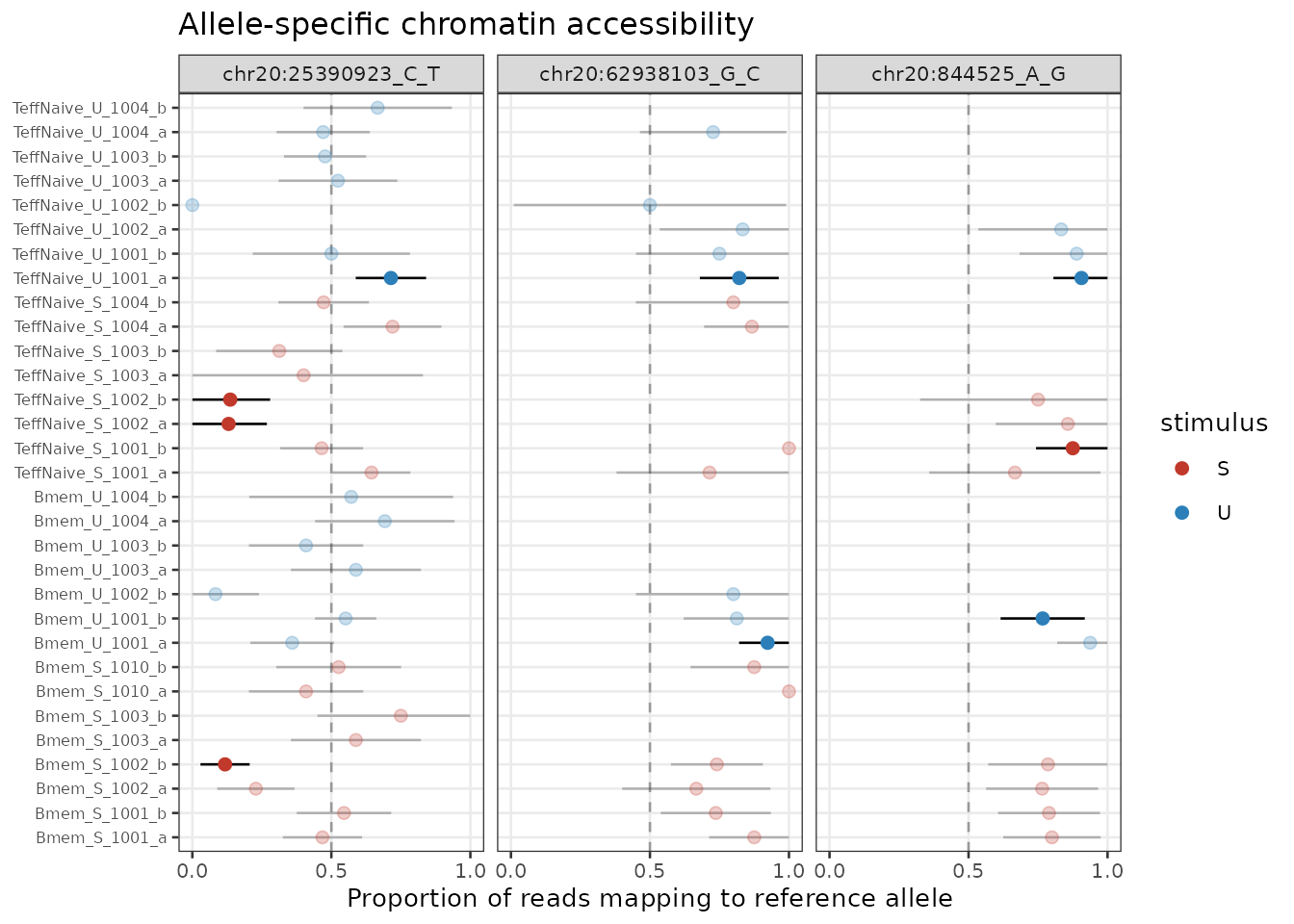

> Warning:  [1m [22m`aes_string()` was deprecated in ggplot2 3.0.0.
>  [36mℹ [39m Please use tidy evaluation idioms with `aes()`.
>  [36mℹ [39m See also `vignette("ggplot2-in-packages")` for more information.
>  [36mℹ [39m The deprecated feature was likely used in the  [34mChrAccR [39m package.
>   Please report the issue at
>    [3m [34m<https://github.com/EpigenomeInformatics/ChrAccR/issues> [39m [23m.
>  [90mThis warning is displayed once every 8 hours. [39m
>  [90mCall `lifecycle::last_lifecycle_warnings()` to see where this warning was [39m
>  [90mgenerated. [39m

plotASCVolcano(dsDemo, stats = ascStats, sigCut = 0.1)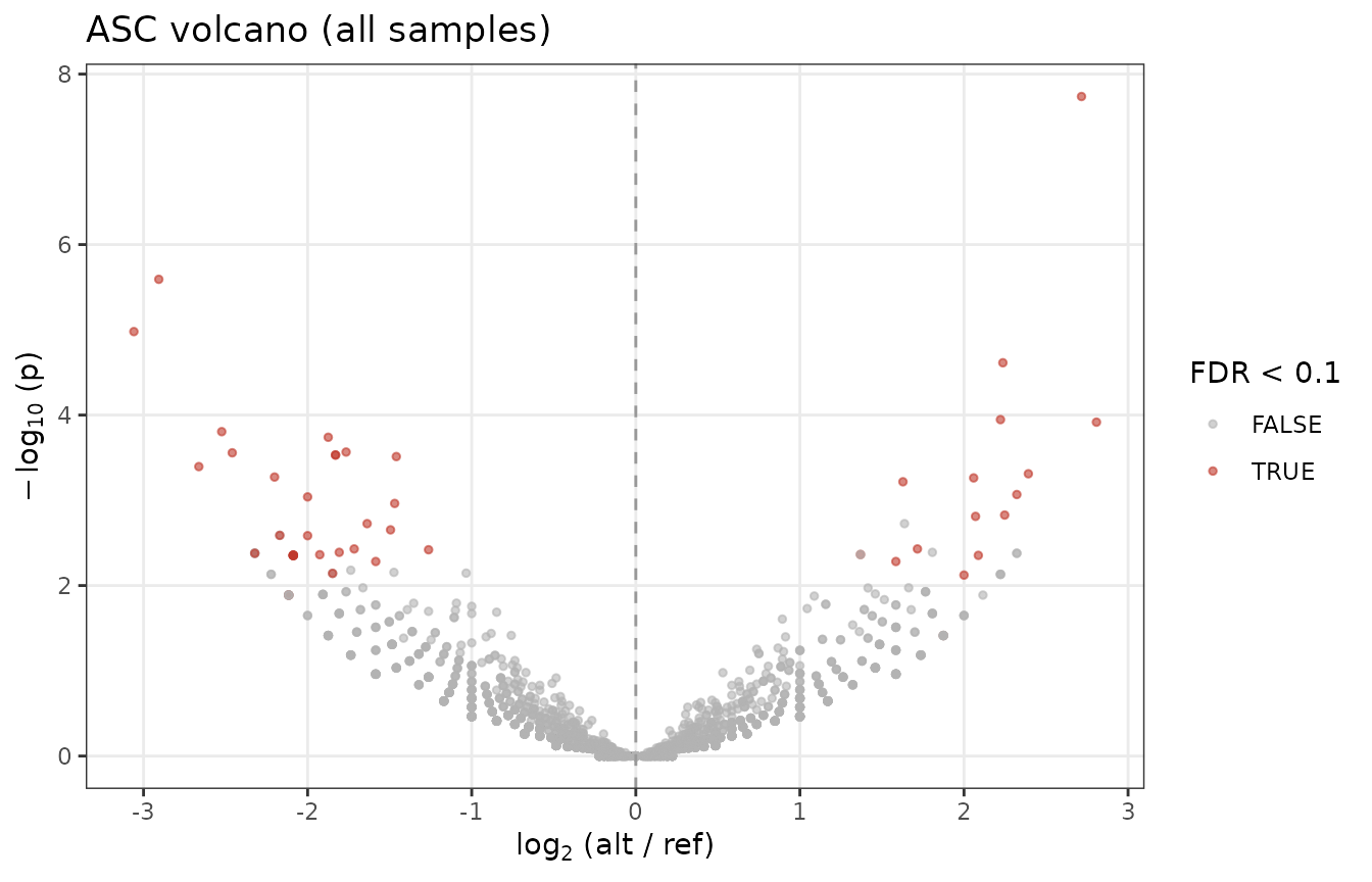

plotASCManhattan(dsDemo, stats = ascStats, sigCut = 0.1)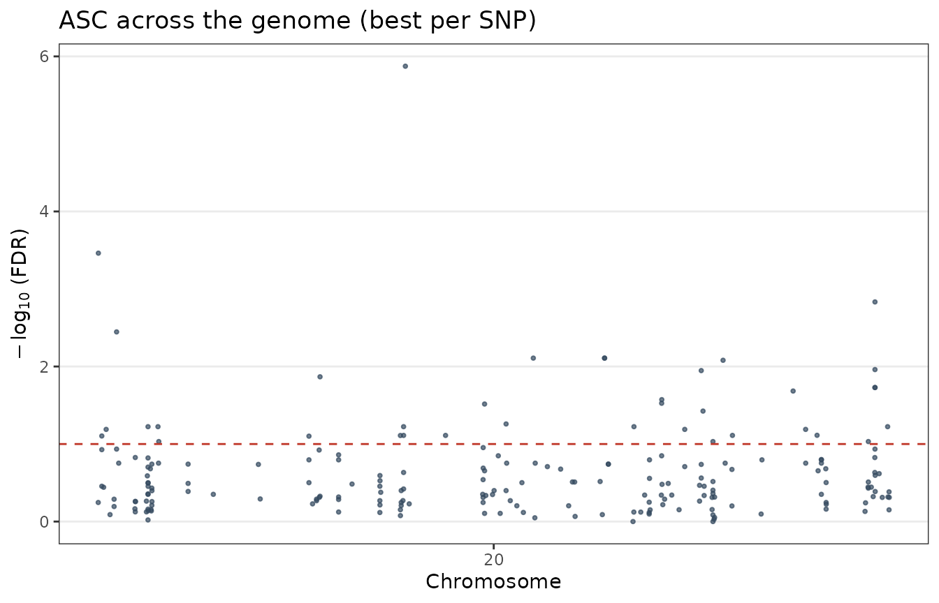

Check where the calls came from before reading anything into them. A donor with deeper libraries contributes more significant sites through power alone, and a donor with a bad genotype batch contributes more because its false heterozygotes all look perfectly imbalanced. Counting the calls per donor shows both.

sigPerDonor <- ascStats[fdr < 0.1, .(nSites = uniqueN(snpId)), by = donor]

ggplot(sigPerDonor, aes(x = reorder(donor, -nSites), y = nSites)) +
  geom_col(fill = "#34495E", width = 0.65) +
  labs(x = "Donor", y = "Significant ASC sites (FDR < 0.1)",
       title = "ASC calls contributed by each donor")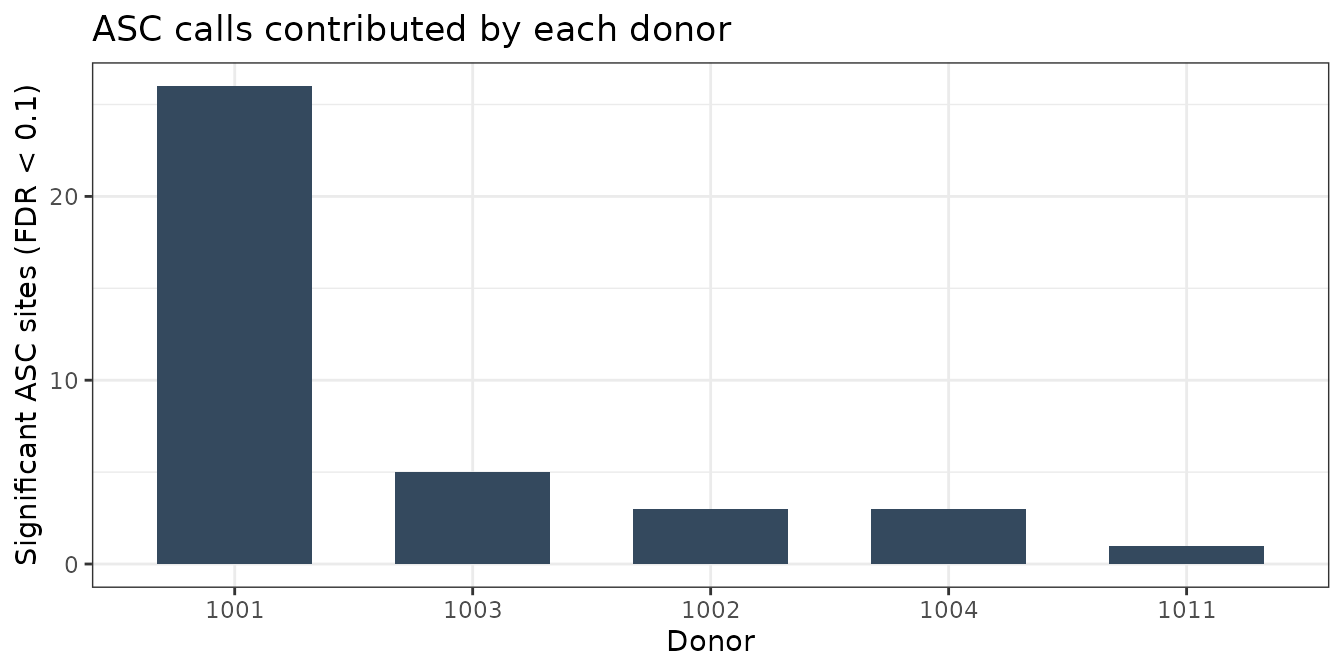

Bars of roughly equal height are fine. One bar several times the rest means going back to that donor’s coverage and genotype QC before trusting sites only it supports.

One significant call in one donor is weak evidence for the same reason. filterForRecurrence() counts how many donors independently support each site.

recurrent <- filterForRecurrence(ascStats, minDonors = 2, fdrCutoff = 0.1)

> 2026-09-03 19:39:31     5.5  STATUS STARTED Identifying Recurrent ASC Sites
> 2026-09-03 19:39:31     5.5    INFO     Initial significant events: 47
> 2026-09-03 19:39:31     5.5    INFO     Recurrent events (N>= 2 donors): 1
> 2026-09-03 19:39:31     5.5  STATUS COMPLETED Identifying Recurrent ASC Sites

head(recurrent, 5)

>                 snpId n_donors_sig mean_LFC
>                <char>        <int>    <num>
> 1: chr20:25390923_C_T            2 1.541855

Every cell type was counted against the same master list, so the per-cell-type objects stack into one aligned pair of matrices.

merged <- mergeDsASCArray(ascDir)

The sharing question is asymmetric. Take the sites significant in cell type A and ask what they do in B: imbalanced in the same direction, balanced, or too shallow to say. ascSharing() separates those three and uses ashr to estimate the proportion with a non-zero effect in B, which is more informative than counting significance calls twice.

cellsPresent <- unique(pooled$annot$cellType)
samplesA <- pooled$annot[cellType == cellsPresent[1], sampleId]
samplesB <- pooled$annot[cellType == cellsPresent[2], sampleId]

aggA <- ascAggregate(pooled$ref, pooled$alt, samplesA)
aggB <- ascAggregate(pooled$ref, pooled$alt, samplesB)

sharing <- ascSharing(aggA$ref, aggA$alt, aggB$ref, aggB$alt,
                      fdrA = 0.01, minReadsB = 4)
sharing

ascSitePosterior() gives the per-site posterior and FDR behind that estimate. ascStratum() labels a pair of groups by whether they share lineage, condition, both or neither. estimateSharedImbalance() runs the same logic directly on two DsASC objects when the matrices have not been merged by hand.

shared <- estimateSharedImbalance(dsTcell, dsBcell, fdrCutoff = 0.01)
shared$sharing_estimate

From sites to motifs

A variant links to a transcription factor through the change in predicted binding. For each site, take a window as wide as the widest motif, substitute the centre base to get the reference and the alternative version, score both with every PWM, and record delta = score(ALT) - score(REF). A positive delta means the alternative allele is the predicted stronger binder.

library(JASPAR2020); library(TFBSTools); library(motifmatchr)
library(BSgenome.Hsapiens.UCSC.hg38)

pfms  <- getMatrixSet(JASPAR2020, list(species = 9606, collection = "CORE"))
flank <- max(vapply(pfms, function(p) ncol(as.matrix(p)), 1L))

sites <- coordDt[snpId %in% sigSnps]
gr    <- GRanges(sites$chrom, IRanges(sites$pos - flank, sites$pos + flank))
seqRef <- getSeq(BSgenome.Hsapiens.UCSC.hg38, gr)
seqAlt <- replaceLetterAt(
  seqRef,
  at = matrix(seq_len(width(seqRef)[1]) == (flank + 1L),
              nrow = length(seqRef), ncol = width(seqRef)[1], byrow = TRUE),
  letter = sites$ALT)

scoreSet <- function(s) as.matrix(motifScores(
  matchMotifs(pfms, s, out = "scores", bg = "even", p.cutoff = 1)))
delta <- scoreSet(seqAlt) - scoreSet(seqRef)
colnames(delta) <- vapply(pfms, name, "")

deltaDt <- rbindlist(lapply(colnames(delta), function(tfName)
  data.table(snpId = sites$snpId, tf = tfName, delta = delta[, tfName])))

Only the ASC-significant sites are scored. That is what keeps a genome-wide motif set affordable, and sites with no imbalance carry no allelic information anyway.

deltaDemo already holds a table of this shape. In the packaged example it is the real output of the code above, computed once over the example sites by the data script. In the simulated fallback it is three profiles: one aligned with the injected imbalance, one partly aligned, one shuffled.

deltaDemo[, .(nSites = .N, meanAbsDelta = round(mean(abs(delta)), 2)), by = tf]

>        tf nSites meanAbsDelta
>    <char>  <int>        <num>
> 1:   CTCF    211         2.27
> 2:  NFKB1    211         2.40
> 3:  GATA3    211         0.85
> 4:   IRF4    211         2.53
> 5:  BACH1    211         1.45
> 6:  FOSL1    211         1.31
> 7:   JUNB    211         1.27
> 8:   SPI1    211         1.61
> 9:   TCF7    211         0.83

Each site is then labelled by the allele its motif prefers. Sites past the threshold in either direction are called for that allele, and everything in between is the internal control. The driver script uses 1.0 on the PWM score; it is lower here because the example carries a few thousand sites rather than a genome’s worth.

prefDelta <- 0.5

prefDt <- data.table::copy(deltaDemo)
prefDt[, preference := fifelse(delta >  prefDelta, "Alternative",
                       fifelse(delta < -prefDelta, "Reference", "No preference"))]
prefDt[, .N, by = .(tf, preference)][order(tf, preference)][1:6]

>        tf    preference     N
>    <char>        <char> <int>
> 1:  BACH1   Alternative    50
> 2:  BACH1 No preference   122
> 3:  BACH1     Reference    39
> 4:   CTCF   Alternative    80
> 5:   CTCF No preference    56
> 6:   CTCF     Reference    75

Binding preference and allelic accessibility

This is where the two halves meet. If a variant really disrupts a binding site, the allele the motif prefers should be the more accessible one, and the effect should be stronger when the factor is active. Pooling reads by condition and plotting the reference-allele fraction against the predicted preference tests that directly, with the no-preference sites at 0.5 as a check that the axis is not simply skewed.

condFrac <- function(cond, label) {
  sids <- intersect(pooled$annot[stimulus == cond, sampleId], colnames(pooled$ref))
  r <- rowSums(pooled$ref[, sids, drop = FALSE])
  a <- rowSums(pooled$alt[, sids, drop = FALSE])
  data.table(snpId = rownames(pooled$ref), refFrac = r / (r + a),
             total = r + a, condition = label)
}

fracDt <- rbindlist(list(condFrac("U", "Resting"), condFrac("S", "Stimulated")))
fracDt <- fracDt[total >= 4]

plotDt <- merge(fracDt, prefDt, by = "snpId", allow.cartesian = TRUE)
plotDt[, preference := factor(preference,
        levels = c("Alternative", "No preference", "Reference"))]
plotDt[, condition := factor(condition, levels = c("Resting", "Stimulated"))]

ggplot(plotDt, aes(x = condition, y = refFrac, fill = preference)) +
  geom_hline(yintercept = 0.5, linetype = "dotted") +
  geom_boxplot(outlier.size = 0.3, position = position_dodge(width = 0.8)) +
  facet_wrap(~ tf) +
  scale_fill_manual(values = c("Alternative" = "#1B9E77",
                               "No preference" = "#D95F02",
                               "Reference" = "#7570B3"), name = NULL) +
  scale_y_continuous(limits = c(0, 1)) +
  labs(x = NULL, y = "Proportion of reads on the reference allele",
       title = "Predicted binding preference vs allelic accessibility") +
  theme(legend.position = "bottom")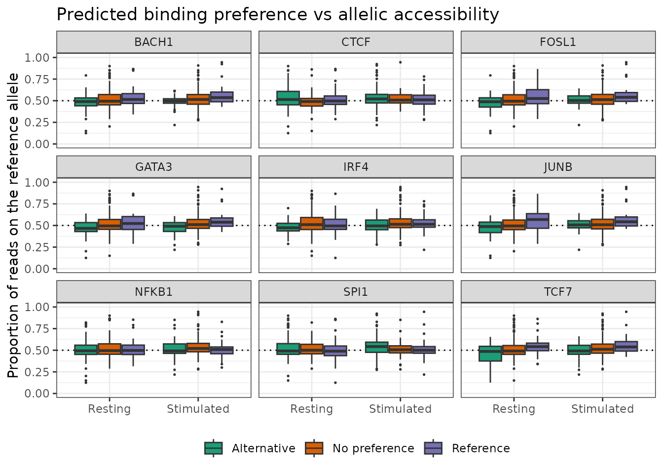

What to look for is separation between the two coloured boxes. Sites where the motif prefers the reference allele should sit above 0.5, sites where it prefers the alternative below it. A Mann-Whitney test per factor and condition puts a number on the gap.

plotDt[preference %in% c("Reference", "Alternative"),
       .(p = tryCatch(wilcox.test(refFrac ~ droplevels(preference))$p.value,
                      error = function(e) NA_real_)),
       by = .(tf, condition)][order(p)]

>         tf  condition           p
>     <char>     <fctr>       <num>
>  1:  BACH1 Stimulated 0.003755054
>  2:   TCF7    Resting 0.009438362
>  3:   TCF7 Stimulated 0.009719738
>  4:   JUNB    Resting 0.011189696
>  5:  GATA3 Stimulated 0.012781993
>  6:   JUNB Stimulated 0.022853598
>  7:  FOSL1 Stimulated 0.025915865
>  8:  BACH1    Resting 0.040652960
>  9:   IRF4    Resting 0.040864317
> 10:  FOSL1    Resting 0.040904532
> 11:   SPI1 Stimulated 0.049796877
> 12:  GATA3    Resting 0.053568619
> 13:   IRF4 Stimulated 0.097353430
> 14:   SPI1    Resting 0.314953736
> 15:   CTCF Stimulated 0.432949012
> 16:   CTCF    Resting 0.498575427
> 17:  NFKB1 Stimulated 0.651486373
> 18:  NFKB1    Resting 0.752118400

droplevels() matters here. preference has three levels, and the formula interface of wilcox.test rejects a grouping factor that still carries an unused level, so without it every p-value comes back as NA through the tryCatch.

Cross-referencing published calls

The calls can be checked against the allele-specific variants in Calderon et al., Nature Genetics 2019 (doi:10.1038/s41588-019-0505-9). Their supplementary table lists genotypes, WASP-corrected counts and allele fractions for the GWAS-overlapping ASC sites. Lifting those coordinates to the working assembly and matching per donor and site answers three questions: whether the direction of imbalance is reproduced, whether the reference fraction at matched sites is skewed relative to theirs, and whether the significant set sits at a comparable allele fraction overall.

Session information

sessionInfo()

> Warning in system("timedatectl", intern = TRUE): running command 'timedatectl'
> had status 1

> R version 4.4.1 (2024-06-14)
> Platform: x86_64-conda-linux-gnu
> Running under: Debian GNU/Linux 11 (bullseye)
> 
> Matrix products: default
> BLAS/LAPACK: /icbb/projects/share/software/packages/miniconda3/envs/alleleSpec/lib/libopenblasp-r0.3.30.so;  LAPACK version 3.12.0
> 
> locale:
>  [1] LC_CTYPE=en_US.UTF-8       LC_NUMERIC=C              
>  [3] LC_TIME=en_US.UTF-8        LC_COLLATE=en_US.UTF-8    
>  [5] LC_MONETARY=en_US.UTF-8    LC_MESSAGES=en_US.UTF-8   
>  [7] LC_PAPER=en_US.UTF-8       LC_NAME=C                 
>  [9] LC_ADDRESS=C               LC_TELEPHONE=C            
> [11] LC_MEASUREMENT=en_US.UTF-8 LC_IDENTIFICATION=C       
> 
> time zone: Europe/Berlin
> tzcode source: system (glibc)
> 
> attached base packages:
> [1] stats4    stats     graphics  grDevices utils     datasets  methods  
> [8] base     
> 
> other attached packages:
> [1] ggplot2_4.0.1        data.table_1.17.8    GenomicRanges_1.58.0
> [4] GenomeInfoDb_1.42.0  IRanges_2.40.0       S4Vectors_0.44.0    
> [7] BiocGenerics_0.52.0  ChrAccR_0.9.26      
> 
> loaded via a namespace (and not attached):
>  [1] SummarizedExperiment_1.36.0 gtable_0.3.6               
>  [3] xfun_0.54                   bslib_0.9.0                
>  [5] htmlwidgets_1.6.4           rhdf5_2.50.0               
>  [7] Biobase_2.66.0              lattice_0.22-7             
>  [9] generics_0.1.4              rhdf5filters_1.18.0        
> [11] vctrs_0.6.5                 tools_4.4.1                
> [13] bitops_1.0-9                parallel_4.4.1             
> [15] tibble_3.3.0                pkgconfig_2.0.3            
> [17] Matrix_1.7-4                RColorBrewer_1.1-3         
> [19] S7_0.2.1                    desc_1.4.3                 
> [21] lifecycle_1.0.4             GenomeInfoDbData_1.2.13    
> [23] compiler_4.4.1              farver_2.1.2               
> [25] Rsamtools_2.22.0            textshaping_1.0.1          
> [27] Biostrings_2.74.0           codetools_0.2-20           
> [29] muLogR_0.2                  muRtools_0.9.6             
> [31] htmltools_0.5.8.1           sass_0.4.10                
> [33] yaml_2.3.11                 pillar_1.11.1              
> [35] pkgdown_2.2.0               crayon_1.5.3               
> [37] jquerylib_0.1.4             BiocParallel_1.40.0        
> [39] DelayedArray_0.32.0         cachem_1.1.0               
> [41] abind_1.4-8                 tidyselect_1.2.1           
> [43] digest_0.6.39               dplyr_1.1.4                
> [45] labeling_0.4.3              fastmap_1.2.0              
> [47] grid_4.4.1                  cli_3.6.5                  
> [49] SparseArray_1.6.0           magrittr_2.0.4             
> [51] S4Arrays_1.6.0              dichromat_2.0-0.1          
> [53] withr_3.0.2                 UCSC.utils_1.2.0           
> [55] scales_1.4.0                rmarkdown_2.30             
> [57] XVector_0.46.0              httr_1.4.7                 
> [59] matrixStats_1.5.0           ragg_1.5.0                 
> [61] HDF5Array_1.34.0            evaluate_1.0.5             
> [63] knitr_1.50                  rlang_1.1.6                
> [65] glue_1.8.0                  jsonlite_2.0.0             
> [67] R6_2.6.1                    Rhdf5lib_1.28.0            
> [69] MatrixGenerics_1.18.0       GenomicAlignments_1.42.0   
> [71] systemfonts_1.3.1           fs_1.6.6                   
> [73] zlibbioc_1.52.0

Allele-specific chromatin accessibility
using ChrAccR

Irem B. Gunduz

2026-09-03

Introduction

The shape of the pipeline

Requirements

Before R: genotypes and bias correction

One site list for every donor

Counting alleles

Restricting to open chromatin

The example dataset

Cleaning before testing

Testing for allelic imbalance

From sites to motifs

Binding preference and allelic accessibility

Cross-referencing published calls

Session information

Allele-specific chromatin accessibility using ChrAccR

Irem B. Gunduz

2026-09-03

Introduction

The shape of the pipeline

Requirements

Before R: genotypes and bias correction

One site list for every donor

Counting alleles

Restricting to open chromatin

The example dataset

Cleaning before testing

Testing for allelic imbalance

Sharing across cell types

From sites to motifs

Binding preference and allelic accessibility

Cross-referencing published calls

Session information

Allele-specific chromatin accessibility
using ChrAccR